Free Statistics

of Irreproducible Research!

Author's title

Author*The author of this computation has been verified*
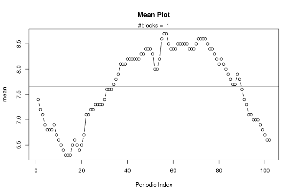
R Software Modulerwasp_meanplot.wasp
Title produced by softwareMean Plot
Date of computationFri, 31 Oct 2008 07:59:49 -0600
Cite this page as followsStatistical Computations at FreeStatistics.org, Office for Research Development and Education, URL https://freestatistics.org/blog/index.php?v=date/2008/Oct/31/t1225461687ueb3xqwnrk3766u.htm/, Retrieved Sat, 18 May 2024 07:24:52 +0000
Statistical Computations at FreeStatistics.org, Office for Research Development and Education, URL https://freestatistics.org/blog/index.php?pk=20281, Retrieved Sat, 18 May 2024 07:24:52 +0000
QR Codes:

Original text written by user:
IsPrivate?No (this computation is public)
User-defined keywords
Estimated Impact168
Family? (F = Feedback message, R = changed R code, M = changed R Module, P = changed Parameters, D = changed Data)
F       [Mean Plot] [Hypothesis Testin...] [2008-10-31 13:59:49] [6797a1f4a60918966297e9d9220cabc2] [Current]
-   PD    [Mean Plot] [blog werkzoekende...] [2008-11-06 14:47:45] [ed2ba3b6182103c15c0ab511ae4e6284]
-   PD    [Mean Plot] [Verbetering Task 5] [2008-11-11 11:02:48] [299afd6311e4c20059ea2f05c8dd029d]
-   PD    [Mean Plot] [asses] [2008-11-11 11:32:21] [74be16979710d4c4e7c6647856088456]
-   PD    [Mean Plot] [verbetering hypot...] [2008-11-11 18:34:25] [063e4b67ad7d3a8a83eccec794cd5aa7]
Feedback Forum
2008-11-06 14:54:43 [Tom Ardies] [reply
Door de blocks gelijk te stellen aan het aantal steekproeven dat je neemt, wordt meanplot eigenlijk gelijk aan je run sequence plot. Om iets te kunnen analyseren moet je de blocks op 12 zetten, zodat elke block een gemiddelde is van elke maand.

De link is je dataset met blocks 12. Tussen periode zes en zeven zie je een duidelijk verschil op de meanplot, dit kan wijzen op seizonaal gedrag.

Als je de notched boxplots bekijkt is er maandelijks bijna geen verschil, tenzij je naar de sequential blocks kijkt. Hier zie je een stijging en dan weer een daling. aangezien je data set over 8 jaar verloopt kan dit te maken hebben met de economische conjuctuur.

http://www.freestatistics.org/blog/index.php?v=date/2008/Nov/06/t1225982927bft4apn1tlbz1pk.htm
2008-11-11 11:35:30 [Stijn Loomans] [reply
Je hebt het aantal blocks gelijkgesteld aan het aantal steekproeven. Waardoor je meanplot eingelijk zinloos wordt. Om het goed te kunnen analyseren had je het aantal block op 12( aantal maanden) moeten zetten. Zodat elke blok het gemmiddelde van een maand is.

Als je dit wel waart gaan doen had je gemerkt dat tussen 6 en 7 er een duidelijk verschil is. Dit kan wijzen op seizonaal gedrag.

http://www.freestatistics.org/blog/date/2008/Nov/11/t1226403172h6dtgztloucc6cb.htm

Als je dan gaat zien naar de notched boxplots is er bijna geen verschil te zien, buiten bij de sequantial blocks. Hier zie je een sterke stijging gevolgd door sterke daling . Dit kan te maken hebben met de economische groei over die 8 jaren heen
2008-11-11 18:39:54 [Ellen Van Ham] [reply
Het aantal blocks werd op 102 (= aantal observaties) gezet. Dit was niet de bedoeling, deze moeten op 12 blijven staan. Door het 102 te zetten wordt de meanplot zinloos.
De juiste conclusie: je ziet een duidelijk verschil tussen 6 en 7. Dit kan onder andere wijzen op seizonaliteit. Zie ook forum voor link.
Bij de notched box plot zien we bijna geen verschillen. Eerst zien we een stijging, gevolgd door een daling. Hierbij moeten we rekening houden met de economische situtuatie over de jaren heen. http://www.freestatistics.org/blog/index.php?v=date/2008/Nov/11/t1226428507pt2fg0k7559mtjx.htm

Post a new message
Dataseries X:
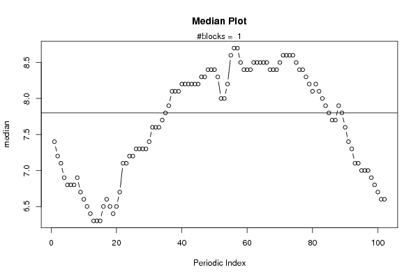
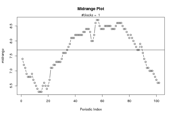
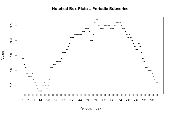
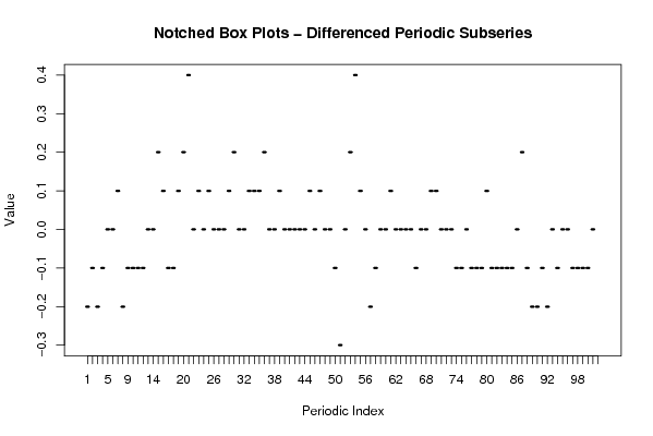
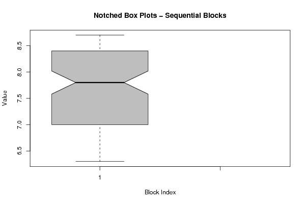
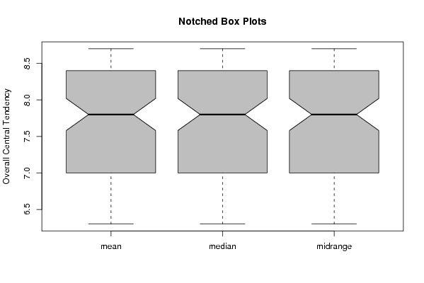
7,4
7,2
7,1
6,9
6,8
6,8
6,8
6,9
6,7
6,6
6,5
6,4
6,3
6,3
6,3
6,5
6,6
6,5
6,4
6,5
6,7
7,1
7,1
7,2
7,2
7,3
7,3
7,3
7,3
7,4
7,6
7,6
7,6
7,7
7,8
7,9
8,1
8,1
8,1
8,2
8,2
8,2
8,2
8,2
8,2
8,3
8,3
8,4
8,4
8,4
8,3
8
8
8,2
8,6
8,7
8,7
8,5
8,4
8,4
8,4
8,5
8,5
8,5
8,5
8,5
8,4
8,4
8,4
8,5
8,6
8,6
8,6
8,6
8,5
8,4
8,4
8,3
8,2
8,1
8,2
8,1
8
7,9
7,8
7,7
7,7
7,9
7,8
7,6
7,4
7,3
7,1
7,1
7
7
7
6,9
6,8
6,7
6,6
6,6


Summary of computational transaction
Raw Inputview raw input (R code)
Raw Outputview raw output of R engine
Computing time5 seconds
R Server'Herman Ole Andreas Wold' @ 193.190.124.10:1001

\begin{tabular}{lllllllll}
\hline
Summary of computational transaction \tabularnewline
Raw Input & view raw input (R code)  \tabularnewline
Raw Output & view raw output of R engine  \tabularnewline
Computing time & 5 seconds \tabularnewline
R Server & 'Herman Ole Andreas Wold' @ 193.190.124.10:1001 \tabularnewline
\hline
\end{tabular}
%Source: https://freestatistics.org/blog/index.php?pk=20281&T=0

[TABLE]
[ROW][C]Summary of computational transaction[/C][/ROW]
[ROW][C]Raw Input[/C][C]view raw input (R code) [/C][/ROW]
[ROW][C]Raw Output[/C][C]view raw output of R engine [/C][/ROW]
[ROW][C]Computing time[/C][C]5 seconds[/C][/ROW]
[ROW][C]R Server[/C][C]'Herman Ole Andreas Wold' @ 193.190.124.10:1001[/C][/ROW]
[/TABLE]
Source: https://freestatistics.org/blog/index.php?pk=20281&T=0

Globally Unique Identifier (entire table): ba.freestatistics.org/blog/index.php?pk=20281&T=0

As an alternative you can also use a QR Code:  

The GUIDs for individual cells are displayed in the table below:

Summary of computational transaction
Raw Inputview raw input (R code)
Raw Outputview raw output of R engine
Computing time5 seconds
R Server'Herman Ole Andreas Wold' @ 193.190.124.10:1001


Parameters (Session):
par1 = 102 ;
Parameters (R input):
par1 = 102 ;
R code (references can be found in the software module):
par1 <- as.numeric(par1)
(n <- length(x))
(np <- floor(n / par1))
arr <- array(NA,dim=c(par1,np+1))
darr <- array(NA,dim=c(par1,np+1))
ari <- array(0,dim=par1)
dx <- diff(x)
j <- 0
for (i in 1:n)
{
j = j + 1
ari[j] = ari[j] + 1
arr[j,ari[j]] <- x[i]
darr[j,ari[j]] <- dx[i]
if (j == par1) j = 0
}
ari
arr
darr
arr.mean <- array(NA,dim=par1)
arr.median <- array(NA,dim=par1)
arr.midrange <- array(NA,dim=par1)
for (j in 1:par1)
{
arr.mean[j] <- mean(arr[j,],na.rm=TRUE)
arr.median[j] <- median(arr[j,],na.rm=TRUE)
arr.midrange[j] <- (quantile(arr[j,],0.75,na.rm=TRUE) + quantile(arr[j,],0.25,na.rm=TRUE)) / 2
}
overall.mean <- mean(x)
overall.median <- median(x)
overall.midrange <- (quantile(x,0.75) + quantile(x,0.25)) / 2
bitmap(file='plot1.png')
plot(arr.mean,type='b',ylab='mean',main='Mean Plot',xlab='Periodic Index')
mtext(paste('#blocks = ',np))
abline(overall.mean,0)
dev.off()
bitmap(file='plot2.png')
plot(arr.median,type='b',ylab='median',main='Median Plot',xlab='Periodic Index')
mtext(paste('#blocks = ',np))
abline(overall.median,0)
dev.off()
bitmap(file='plot3.png')
plot(arr.midrange,type='b',ylab='midrange',main='Midrange Plot',xlab='Periodic Index')
mtext(paste('#blocks = ',np))
abline(overall.midrange,0)
dev.off()
bitmap(file='plot4.png')
z <- data.frame(t(arr))
names(z) <- c(1:par1)
(boxplot(z,notch=TRUE,col='grey',xlab='Periodic Index',ylab='Value',main='Notched Box Plots - Periodic Subseries'))
dev.off()
bitmap(file='plot4b.png')
z <- data.frame(t(darr))
names(z) <- c(1:par1)
(boxplot(z,notch=TRUE,col='grey',xlab='Periodic Index',ylab='Value',main='Notched Box Plots - Differenced Periodic Subseries'))
dev.off()
bitmap(file='plot5.png')
z <- data.frame(arr)
names(z) <- c(1:np)
(boxplot(z,notch=TRUE,col='grey',xlab='Block Index',ylab='Value',main='Notched Box Plots - Sequential Blocks'))
dev.off()
bitmap(file='plot6.png')
z <- data.frame(cbind(arr.mean,arr.median,arr.midrange))
names(z) <- list('mean','median','midrange')
(boxplot(z,notch=TRUE,col='grey',ylab='Overall Central Tendency',main='Notched Box Plots'))
dev.off()