Free Statistics
of Irreproducible Research!
Description of Statistical Computation | |||||||||||||||||||||
|---|---|---|---|---|---|---|---|---|---|---|---|---|---|---|---|---|---|---|---|---|---|
| Author's title | |||||||||||||||||||||
| Author | *The author of this computation has been verified* | ||||||||||||||||||||
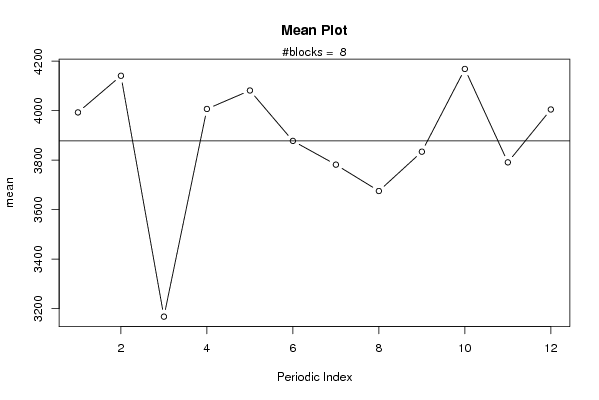
| R Software Module | rwasp_meanplot.wasp | ||||||||||||||||||||
| Title produced by software | Mean Plot | ||||||||||||||||||||
| Date of computation | Thu, 30 Oct 2008 11:43:37 -0600 | ||||||||||||||||||||
| Cite this page as follows | Statistical Computations at FreeStatistics.org, Office for Research Development and Education, URL https://freestatistics.org/blog/index.php?v=date/2008/Oct/30/t1225388659dyk48b5i7ds6fdz.htm/, Retrieved Sat, 18 May 2024 00:51:14 +0000 | ||||||||||||||||||||
| Statistical Computations at FreeStatistics.org, Office for Research Development and Education, URL https://freestatistics.org/blog/index.php?pk=20139, Retrieved Sat, 18 May 2024 00:51:14 +0000 | |||||||||||||||||||||
| QR Codes: | |||||||||||||||||||||
|
| |||||||||||||||||||||
| Original text written by user: | |||||||||||||||||||||
| IsPrivate? | No (this computation is public) | ||||||||||||||||||||
| User-defined keywords | |||||||||||||||||||||
| Estimated Impact | 175 | ||||||||||||||||||||
Tree of Dependent Computations | |||||||||||||||||||||
| Family? (F = Feedback message, R = changed R code, M = changed R Module, P = changed Parameters, D = changed Data) | |||||||||||||||||||||
| F [Mean Plot] [workshop 3] [2007-10-26 12:14:28] [e9ffc5de6f8a7be62f22b142b5b6b1a8] F D [Mean Plot] [Q2:Mean plot] [2008-10-30 13:08:02] [1ce0d16c8f4225c977b42c8fa93bc163] F D [Mean Plot] [Task 5(2)] [2008-10-30 17:43:37] [8758b22b4a10c08c31202f233362e983] [Current] F D [Mean Plot] [Task 5] [2008-11-03 22:14:36] [76963dc1903f0f612b6153510a3818cf] | |||||||||||||||||||||
| Feedback Forum | |||||||||||||||||||||
Post a new message | |||||||||||||||||||||
Dataset | |||||||||||||||||||||
| Dataseries X: | |||||||||||||||||||||
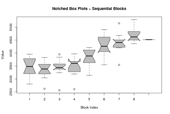
3202,1 3650,2 2805,1 3957,5 3941,3 3905,4 3546,9 3208,7 3402 3661,1 3073,9 3419,2 3532,8 3693,1 2622,9 3130,8 3487,5 3349,7 3044,2 3266 3351,5 3606,8 3419,5 3829,5 3505,1 3845,3 2566,6 3658,5 3954 3460,1 3454,1 3412,8 3418 3349,5 3423,4 3242,8 3277,2 3833 2606,3 3643,8 3686,4 3281,6 3669,3 3191,5 3512,7 3970,7 3601,2 3610 4172,1 3956,2 3142,7 3884,3 3892,2 3613 3730,5 3481,3 3649,5 4215,2 4066,6 4196,8 4536,6 4441,6 3548,3 4735,9 4130,6 4356,2 4159,6 3988 4167,8 4902,2 3909,4 4697,6 4308,9 4420,4 3544,2 4433 4479,7 4533,2 4237,5 4207,4 4394 5148,4 4202,2 4682,5 4884,3 5288,9 4505,2 4611,5 5081,1 4523,1 4412,8 4647,4 4778,6 4495,3 4633,5 4360,5 4517,9 | |||||||||||||||||||||
Tables (Output of Computation) | |||||||||||||||||||||
| |||||||||||||||||||||
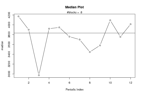
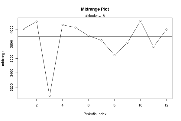
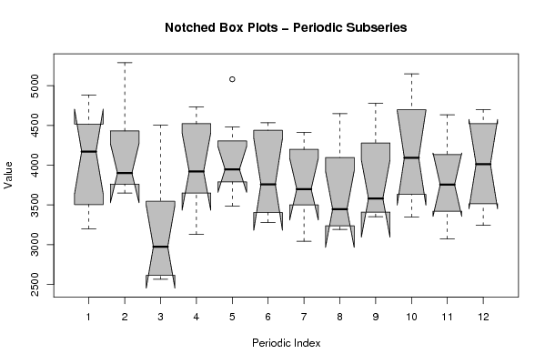
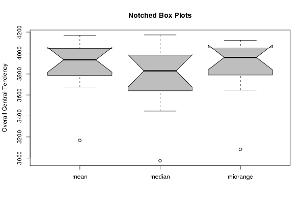
Figures (Output of Computation) | |||||||||||||||||||||
Input Parameters & R Code | |||||||||||||||||||||
| Parameters (Session): | |||||||||||||||||||||
| par1 = 12 ; | |||||||||||||||||||||
| Parameters (R input): | |||||||||||||||||||||
| par1 = 12 ; | |||||||||||||||||||||
| R code (references can be found in the software module): | |||||||||||||||||||||
par1 <- as.numeric(par1) | |||||||||||||||||||||