Free Statistics
of Irreproducible Research!
Description of Statistical Computation | |||||||||||||||||||||
|---|---|---|---|---|---|---|---|---|---|---|---|---|---|---|---|---|---|---|---|---|---|
| Author's title | |||||||||||||||||||||
| Author | *The author of this computation has been verified* | ||||||||||||||||||||
| R Software Module | rwasp_meanplot.wasp | ||||||||||||||||||||
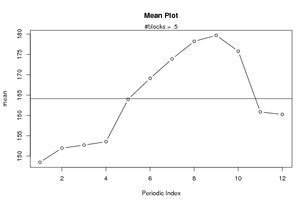
| Title produced by software | Mean Plot | ||||||||||||||||||||
| Date of computation | Wed, 29 Oct 2008 13:39:41 -0600 | ||||||||||||||||||||
| Cite this page as follows | Statistical Computations at FreeStatistics.org, Office for Research Development and Education, URL https://freestatistics.org/blog/index.php?v=date/2008/Oct/29/t1225309258s5x80myt7cswqbr.htm/, Retrieved Fri, 04 Jul 2025 04:02:23 +0000 | ||||||||||||||||||||
| Statistical Computations at FreeStatistics.org, Office for Research Development and Education, URL https://freestatistics.org/blog/index.php?pk=19946, Retrieved Fri, 04 Jul 2025 04:02:23 +0000 | |||||||||||||||||||||
| QR Codes: | |||||||||||||||||||||
|
| |||||||||||||||||||||
| Original text written by user: | |||||||||||||||||||||
| IsPrivate? | No (this computation is public) | ||||||||||||||||||||
| User-defined keywords | |||||||||||||||||||||
| Estimated Impact | 256 | ||||||||||||||||||||
Tree of Dependent Computations | |||||||||||||||||||||
| Family? (F = Feedback message, R = changed R code, M = changed R Module, P = changed Parameters, D = changed Data) | |||||||||||||||||||||
| F [Mean Plot] [workshop 3] [2007-10-26 12:14:28] [e9ffc5de6f8a7be62f22b142b5b6b1a8] F R D [Mean Plot] [Mean Plot] [2008-10-29 16:50:18] [b518240a1c80d4f939bf8b3e34f77cec] F D [Mean Plot] [Totale prijs van ...] [2008-10-29 19:39:41] [6aa66640011d9b98524a5838bcf7301d] [Current] | |||||||||||||||||||||
| Feedback Forum | |||||||||||||||||||||
Post a new message | |||||||||||||||||||||
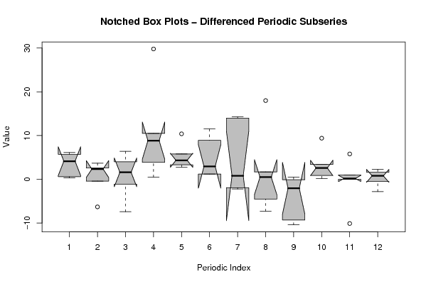
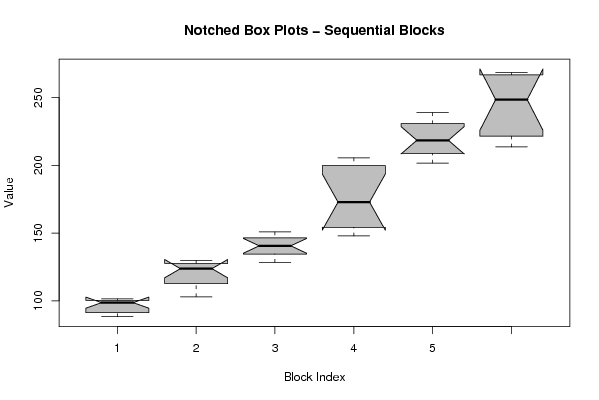
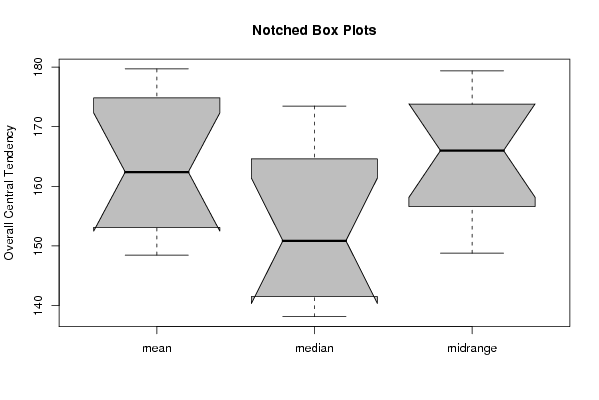
Dataset | |||||||||||||||||||||
| Dataseries X: | |||||||||||||||||||||
88,3 88,6 91 91,5 95,4 98,7 99,9 98,6 100,3 100,2 100,4 101,4 103 109,1 111,4 114,1 121,8 127,6 129,9 128 123,5 124 127,4 127,6 128,4 131,4 135,1 134 144,5 147,3 150,9 148,7 141,4 138,9 139,8 145,6 147,9 148,5 151,1 157,5 167,5 172,3 173,5 187,5 205,5 195,1 204,5 204,5 201,7 207 206,6 210,6 211,1 215 223,9 238,2 238,9 229,6 232,2 222,1 221,6 227,3 221 213,6 243,4 253,8 265,3 268,2 268,5 266,9 | |||||||||||||||||||||
Tables (Output of Computation) | |||||||||||||||||||||
| |||||||||||||||||||||
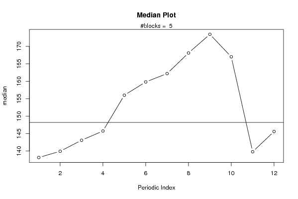
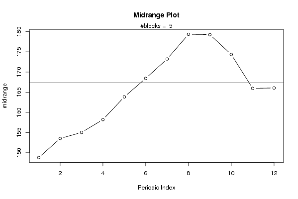
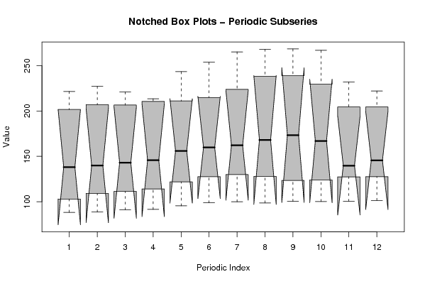
Figures (Output of Computation) | |||||||||||||||||||||
Input Parameters & R Code | |||||||||||||||||||||
| Parameters (Session): | |||||||||||||||||||||
| par1 = 12 ; | |||||||||||||||||||||
| Parameters (R input): | |||||||||||||||||||||
| par1 = 12 ; | |||||||||||||||||||||
| R code (references can be found in the software module): | |||||||||||||||||||||
par1 <- as.numeric(par1) | |||||||||||||||||||||