Free Statistics
of Irreproducible Research!
Description of Statistical Computation | |||||||||||||||||||||||||||||||||||||||||||||||||||||||||||||||||||||||||||||||||||||||||||||||||||||||||||||||||||||||||||||||||
|---|---|---|---|---|---|---|---|---|---|---|---|---|---|---|---|---|---|---|---|---|---|---|---|---|---|---|---|---|---|---|---|---|---|---|---|---|---|---|---|---|---|---|---|---|---|---|---|---|---|---|---|---|---|---|---|---|---|---|---|---|---|---|---|---|---|---|---|---|---|---|---|---|---|---|---|---|---|---|---|---|---|---|---|---|---|---|---|---|---|---|---|---|---|---|---|---|---|---|---|---|---|---|---|---|---|---|---|---|---|---|---|---|---|---|---|---|---|---|---|---|---|---|---|---|---|---|---|---|---|
| Author's title | |||||||||||||||||||||||||||||||||||||||||||||||||||||||||||||||||||||||||||||||||||||||||||||||||||||||||||||||||||||||||||||||||
| Author | *The author of this computation has been verified* | ||||||||||||||||||||||||||||||||||||||||||||||||||||||||||||||||||||||||||||||||||||||||||||||||||||||||||||||||||||||||||||||||
| R Software Module | rwasp_smp.wasp | ||||||||||||||||||||||||||||||||||||||||||||||||||||||||||||||||||||||||||||||||||||||||||||||||||||||||||||||||||||||||||||||||
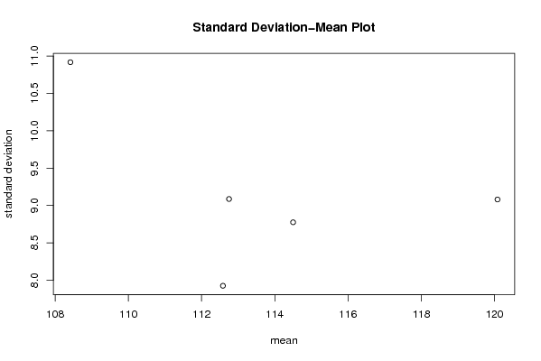
| Title produced by software | Standard Deviation-Mean Plot | ||||||||||||||||||||||||||||||||||||||||||||||||||||||||||||||||||||||||||||||||||||||||||||||||||||||||||||||||||||||||||||||||
| Date of computation | Thu, 27 Nov 2008 15:08:29 -0700 | ||||||||||||||||||||||||||||||||||||||||||||||||||||||||||||||||||||||||||||||||||||||||||||||||||||||||||||||||||||||||||||||||
| Cite this page as follows | Statistical Computations at FreeStatistics.org, Office for Research Development and Education, URL https://freestatistics.org/blog/index.php?v=date/2008/Nov/27/t1227823771vx1agprqpqxculh.htm/, Retrieved Sun, 19 May 2024 11:49:37 +0000 | ||||||||||||||||||||||||||||||||||||||||||||||||||||||||||||||||||||||||||||||||||||||||||||||||||||||||||||||||||||||||||||||||
| Statistical Computations at FreeStatistics.org, Office for Research Development and Education, URL https://freestatistics.org/blog/index.php?pk=25921, Retrieved Sun, 19 May 2024 11:49:37 +0000 | |||||||||||||||||||||||||||||||||||||||||||||||||||||||||||||||||||||||||||||||||||||||||||||||||||||||||||||||||||||||||||||||||
| QR Codes: | |||||||||||||||||||||||||||||||||||||||||||||||||||||||||||||||||||||||||||||||||||||||||||||||||||||||||||||||||||||||||||||||||
|
| |||||||||||||||||||||||||||||||||||||||||||||||||||||||||||||||||||||||||||||||||||||||||||||||||||||||||||||||||||||||||||||||||
| Original text written by user: | |||||||||||||||||||||||||||||||||||||||||||||||||||||||||||||||||||||||||||||||||||||||||||||||||||||||||||||||||||||||||||||||||
| IsPrivate? | No (this computation is public) | ||||||||||||||||||||||||||||||||||||||||||||||||||||||||||||||||||||||||||||||||||||||||||||||||||||||||||||||||||||||||||||||||
| User-defined keywords | |||||||||||||||||||||||||||||||||||||||||||||||||||||||||||||||||||||||||||||||||||||||||||||||||||||||||||||||||||||||||||||||||
| Estimated Impact | 227 | ||||||||||||||||||||||||||||||||||||||||||||||||||||||||||||||||||||||||||||||||||||||||||||||||||||||||||||||||||||||||||||||||
Tree of Dependent Computations | |||||||||||||||||||||||||||||||||||||||||||||||||||||||||||||||||||||||||||||||||||||||||||||||||||||||||||||||||||||||||||||||||
| Family? (F = Feedback message, R = changed R code, M = changed R Module, P = changed Parameters, D = changed Data) | |||||||||||||||||||||||||||||||||||||||||||||||||||||||||||||||||||||||||||||||||||||||||||||||||||||||||||||||||||||||||||||||||
| F [Law of Averages] [Random Walk Simul...] [2008-11-25 18:40:39] [b98453cac15ba1066b407e146608df68] F [Law of Averages] [Random Walk Simul...] [2008-11-27 19:45:04] [58bf45a666dc5198906262e8815a9722] F RMPD [Standard Deviation-Mean Plot] [Standard Deviatio...] [2008-11-27 22:08:29] [63db34dadd44fb018112addcdefe949f] [Current] - D [Standard Deviation-Mean Plot] [Standard Deviatio...] [2008-11-27 22:18:06] [58bf45a666dc5198906262e8815a9722] - RMP [(Partial) Autocorrelation Function] [(Partial) Autocor...] [2008-11-27 22:25:58] [58bf45a666dc5198906262e8815a9722] F P [(Partial) Autocorrelation Function] [(Partial) Autocor...] [2008-11-28 10:12:46] [58bf45a666dc5198906262e8815a9722] F P [(Partial) Autocorrelation Function] [(Partial) Autocor...] [2008-11-28 10:15:39] [58bf45a666dc5198906262e8815a9722] F P [(Partial) Autocorrelation Function] [(Partial) Autocor...] [2008-11-28 10:17:42] [58bf45a666dc5198906262e8815a9722] F P [(Partial) Autocorrelation Function] [(Partial) Autocor...] [2008-11-28 10:20:24] [58bf45a666dc5198906262e8815a9722] - PD [(Partial) Autocorrelation Function] [(Partial) Autocor...] [2008-11-28 10:23:41] [58bf45a666dc5198906262e8815a9722] - PD [(Partial) Autocorrelation Function] [(Partial) Autocor...] [2008-11-28 10:26:03] [58bf45a666dc5198906262e8815a9722] - PD [(Partial) Autocorrelation Function] [(Partial) Autocor...] [2008-11-28 10:26:03] [58bf45a666dc5198906262e8815a9722] - PD [(Partial) Autocorrelation Function] [(Partial) Autocor...] [2008-11-28 10:29:39] [58bf45a666dc5198906262e8815a9722] - PD [(Partial) Autocorrelation Function] [(Partial) Autocor...] [2008-11-28 10:31:19] [58bf45a666dc5198906262e8815a9722] - RMP [(Partial) Autocorrelation Function] [(Partial) Autocor...] [2008-11-27 22:29:15] [58bf45a666dc5198906262e8815a9722] - RMP [(Partial) Autocorrelation Function] [(Partial) Autocor...] [2008-11-27 22:31:47] [58bf45a666dc5198906262e8815a9722] - RMP [(Partial) Autocorrelation Function] [(Partial) Autocor...] [2008-11-27 22:33:51] [58bf45a666dc5198906262e8815a9722] - RMPD [(Partial) Autocorrelation Function] [(Partial) Autocor...] [2008-11-27 22:37:06] [58bf45a666dc5198906262e8815a9722] - RMPD [(Partial) Autocorrelation Function] [(Partial) Autocor...] [2008-11-27 22:39:04] [58bf45a666dc5198906262e8815a9722] - RMPD [(Partial) Autocorrelation Function] [(Partial) Autocor...] [2008-11-27 22:41:03] [58bf45a666dc5198906262e8815a9722] - RMPD [(Partial) Autocorrelation Function] [(Partial) Autocor...] [2008-11-27 22:42:39] [58bf45a666dc5198906262e8815a9722] - RM D [Variance Reduction Matrix] [Variance Reductio...] [2008-11-27 22:45:11] [58bf45a666dc5198906262e8815a9722] F RM [Variance Reduction Matrix] [Variance Reductio...] [2008-11-27 22:46:51] [58bf45a666dc5198906262e8815a9722] F RMP [Spectral Analysis] [Spectral Analysis...] [2008-11-27 22:49:42] [58bf45a666dc5198906262e8815a9722] - RMP [Spectral Analysis] [Spectral Analysis...] [2008-11-27 22:53:13] [58bf45a666dc5198906262e8815a9722] - RMP [Spectral Analysis] [Spectral Analysis...] [2008-11-27 22:55:39] [58bf45a666dc5198906262e8815a9722] - RMP [Spectral Analysis] [Spectral Analysis...] [2008-11-27 22:58:38] [58bf45a666dc5198906262e8815a9722] - RMPD [Spectral Analysis] [Spectral Analysis...] [2008-11-27 23:01:45] [58bf45a666dc5198906262e8815a9722] - RMPD [Spectral Analysis] [Spectral Analysis...] [2008-11-27 23:04:22] [58bf45a666dc5198906262e8815a9722] - R P [Spectral Analysis] [Q4] [2008-12-01 15:46:23] [84dda5145c389bd11bcc662bd33fe4ba] F R P [Spectral Analysis] [Q4] [2008-12-01 15:46:23] [84dda5145c389bd11bcc662bd33fe4ba] F P [Spectral Analysis] [Q4] [2008-12-01 15:52:17] [43d870b30ac8a7afeb5de9ee11dcfc1a] | |||||||||||||||||||||||||||||||||||||||||||||||||||||||||||||||||||||||||||||||||||||||||||||||||||||||||||||||||||||||||||||||||
| Feedback Forum | |||||||||||||||||||||||||||||||||||||||||||||||||||||||||||||||||||||||||||||||||||||||||||||||||||||||||||||||||||||||||||||||||
Post a new message | |||||||||||||||||||||||||||||||||||||||||||||||||||||||||||||||||||||||||||||||||||||||||||||||||||||||||||||||||||||||||||||||||
Dataset | |||||||||||||||||||||||||||||||||||||||||||||||||||||||||||||||||||||||||||||||||||||||||||||||||||||||||||||||||||||||||||||||||
| Dataseries X: | |||||||||||||||||||||||||||||||||||||||||||||||||||||||||||||||||||||||||||||||||||||||||||||||||||||||||||||||||||||||||||||||||
106 82 114 118 105 105 103 107 123 112 104 122 108 94 120 118 117 113 106 108 122 115 110 120 104 96 121 111 120 114 107 108 127 105 119 121 106 97 119 122 121 106 114 112 127 109 118 123 115 105 116 131 121 104 127 126 124 132 117 123 | |||||||||||||||||||||||||||||||||||||||||||||||||||||||||||||||||||||||||||||||||||||||||||||||||||||||||||||||||||||||||||||||||
Tables (Output of Computation) | |||||||||||||||||||||||||||||||||||||||||||||||||||||||||||||||||||||||||||||||||||||||||||||||||||||||||||||||||||||||||||||||||
| |||||||||||||||||||||||||||||||||||||||||||||||||||||||||||||||||||||||||||||||||||||||||||||||||||||||||||||||||||||||||||||||||
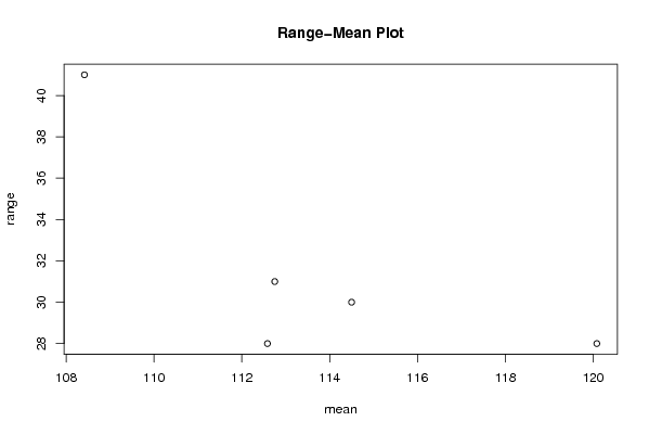
Figures (Output of Computation) | |||||||||||||||||||||||||||||||||||||||||||||||||||||||||||||||||||||||||||||||||||||||||||||||||||||||||||||||||||||||||||||||||
Input Parameters & R Code | |||||||||||||||||||||||||||||||||||||||||||||||||||||||||||||||||||||||||||||||||||||||||||||||||||||||||||||||||||||||||||||||||
| Parameters (Session): | |||||||||||||||||||||||||||||||||||||||||||||||||||||||||||||||||||||||||||||||||||||||||||||||||||||||||||||||||||||||||||||||||
| par1 = 12 ; | |||||||||||||||||||||||||||||||||||||||||||||||||||||||||||||||||||||||||||||||||||||||||||||||||||||||||||||||||||||||||||||||||
| Parameters (R input): | |||||||||||||||||||||||||||||||||||||||||||||||||||||||||||||||||||||||||||||||||||||||||||||||||||||||||||||||||||||||||||||||||
| par1 = 12 ; | |||||||||||||||||||||||||||||||||||||||||||||||||||||||||||||||||||||||||||||||||||||||||||||||||||||||||||||||||||||||||||||||||
| R code (references can be found in the software module): | |||||||||||||||||||||||||||||||||||||||||||||||||||||||||||||||||||||||||||||||||||||||||||||||||||||||||||||||||||||||||||||||||
par1 <- as.numeric(par1) | |||||||||||||||||||||||||||||||||||||||||||||||||||||||||||||||||||||||||||||||||||||||||||||||||||||||||||||||||||||||||||||||||