Free Statistics
of Irreproducible Research!
Description of Statistical Computation | |||||||||||||||||||||
|---|---|---|---|---|---|---|---|---|---|---|---|---|---|---|---|---|---|---|---|---|---|
| Author's title | |||||||||||||||||||||
| Author | *The author of this computation has been verified* | ||||||||||||||||||||
| R Software Module | rwasp_cloud.wasp | ||||||||||||||||||||
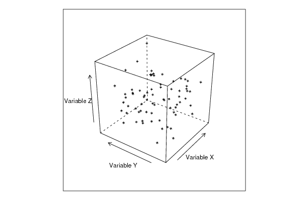
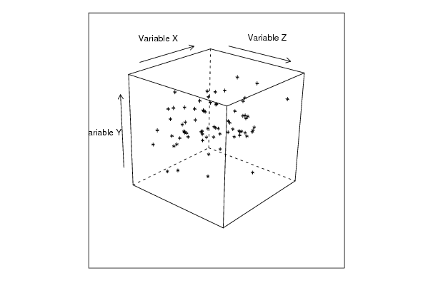
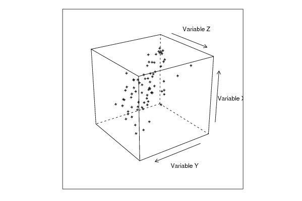
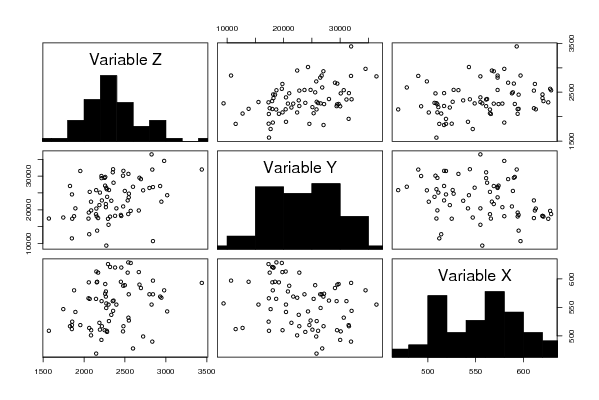
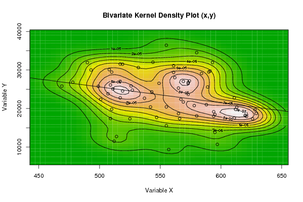
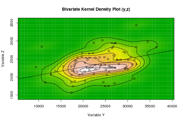
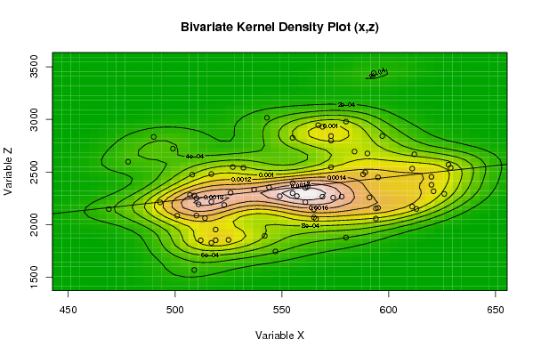
| Title produced by software | Trivariate Scatterplots | ||||||||||||||||||||
| Date of computation | Tue, 11 Nov 2008 02:37:17 -0700 | ||||||||||||||||||||
| Cite this page as follows | Statistical Computations at FreeStatistics.org, Office for Research Development and Education, URL https://freestatistics.org/blog/index.php?v=date/2008/Nov/11/t1226396346g9pcj996yg6ajtr.htm/, Retrieved Sun, 19 May 2024 12:06:05 +0000 | ||||||||||||||||||||
| Statistical Computations at FreeStatistics.org, Office for Research Development and Education, URL https://freestatistics.org/blog/index.php?pk=23250, Retrieved Sun, 19 May 2024 12:06:05 +0000 | |||||||||||||||||||||
| QR Codes: | |||||||||||||||||||||
|
| |||||||||||||||||||||
| Original text written by user: | |||||||||||||||||||||
| IsPrivate? | No (this computation is public) | ||||||||||||||||||||
| User-defined keywords | |||||||||||||||||||||
| Estimated Impact | 177 | ||||||||||||||||||||
Tree of Dependent Computations | |||||||||||||||||||||
| Family? (F = Feedback message, R = changed R code, M = changed R Module, P = changed Parameters, D = changed Data) | |||||||||||||||||||||
| F [Trivariate Scatterplots] [Werkloosheid/insc...] [2008-11-10 16:29:40] [57fa5e3679c393aa19449b2f1be9928b] - [Trivariate Scatterplots] [] [2008-11-11 09:37:17] [19ef54504342c1b076371d395a2ab19f] [Current] | |||||||||||||||||||||
| Feedback Forum | |||||||||||||||||||||
Post a new message | |||||||||||||||||||||
Dataset | |||||||||||||||||||||
| Dataseries X: | |||||||||||||||||||||
517 525 523 519 509 512 519 517 510 509 501 507 569 580 578 565 547 555 562 561 555 544 537 543 594 611 613 611 594 595 591 589 584 573 567 569 621 629 628 612 595 597 593 590 580 574 573 573 620 626 620 588 566 557 561 549 532 526 511 499 555 565 542 527 510 514 517 508 493 490 469 478 | |||||||||||||||||||||
| Dataseries Y: | |||||||||||||||||||||
22780 17351 21382 24561 17409 11514 31514 27071 29462 26105 22397 23843 21705 18089 20764 25316 17704 15548 28029 29383 36438 32034 22679 24319 18004 17537 20366 22782 19169 13807 29743 25591 29096 26482 22405 27044 17970 18730 19684 19785 18479 10698 31956 29506 34506 27165 26736 23691 18157 17328 18205 20995 17382 9367 31124 26551 30651 25859 25100 25778 20418 18688 20424 24776 19814 12738 31566 30111 30019 31934 25826 26835 | |||||||||||||||||||||
| Dataseries Z: | |||||||||||||||||||||
2218 1855 2187 1852 1570 1851 1954 1828 2251 2277 2085 2282 2266 1878 2267 2069 1746 2299 2360 2214 2825 2355 2333 3016 2155 2172 2150 2533 2058 2160 2259 2498 2695 2799 2945 2930 2318 2540 2570 2669 2450 2842 3439 2677 2979 2257 2842 2546 2455 2293 2379 2478 2054 2272 2351 2271 2542 2304 2194 2722 2395 2146 1894 2548 2087 2063 2481 2476 2212 2834 2148 2598 | |||||||||||||||||||||
Tables (Output of Computation) | |||||||||||||||||||||
| |||||||||||||||||||||
Figures (Output of Computation) | |||||||||||||||||||||
Input Parameters & R Code | |||||||||||||||||||||
| Parameters (Session): | |||||||||||||||||||||
| par1 = 50 ; par2 = 50 ; par3 = Y ; par4 = Y ; par5 = Variable X ; par6 = Variable Y ; par7 = Variable Z ; | |||||||||||||||||||||
| Parameters (R input): | |||||||||||||||||||||
| par1 = 50 ; par2 = 50 ; par3 = Y ; par4 = Y ; par5 = Variable X ; par6 = Variable Y ; par7 = Variable Z ; par8 = ; par9 = ; par10 = ; par11 = ; par12 = ; par13 = ; par14 = ; par15 = ; par16 = ; par17 = ; par18 = ; par19 = ; par20 = ; | |||||||||||||||||||||
| R code (references can be found in the software module): | |||||||||||||||||||||
x <- array(x,dim=c(length(x),1)) | |||||||||||||||||||||