Free Statistics
of Irreproducible Research!
Description of Statistical Computation | |||||||||||||||||||||||||||||||||||||||||||||
|---|---|---|---|---|---|---|---|---|---|---|---|---|---|---|---|---|---|---|---|---|---|---|---|---|---|---|---|---|---|---|---|---|---|---|---|---|---|---|---|---|---|---|---|---|---|
| Author's title | |||||||||||||||||||||||||||||||||||||||||||||
| Author | *The author of this computation has been verified* | ||||||||||||||||||||||||||||||||||||||||||||
| R Software Module | rwasp_bidensity.wasp | ||||||||||||||||||||||||||||||||||||||||||||
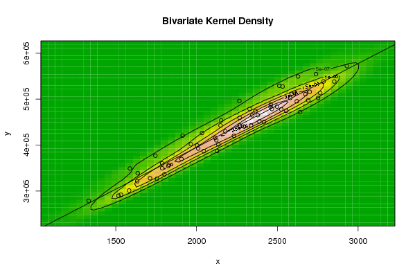
| Title produced by software | Bivariate Kernel Density Estimation | ||||||||||||||||||||||||||||||||||||||||||||
| Date of computation | Sun, 09 Nov 2008 14:12:27 -0700 | ||||||||||||||||||||||||||||||||||||||||||||
| Cite this page as follows | Statistical Computations at FreeStatistics.org, Office for Research Development and Education, URL https://freestatistics.org/blog/index.php?v=date/2008/Nov/09/t1226265196nomsln6lv9mu9ud.htm/, Retrieved Sun, 19 May 2024 09:09:34 +0000 | ||||||||||||||||||||||||||||||||||||||||||||
| Statistical Computations at FreeStatistics.org, Office for Research Development and Education, URL https://freestatistics.org/blog/index.php?pk=22878, Retrieved Sun, 19 May 2024 09:09:34 +0000 | |||||||||||||||||||||||||||||||||||||||||||||
| QR Codes: | |||||||||||||||||||||||||||||||||||||||||||||
|
| |||||||||||||||||||||||||||||||||||||||||||||
| Original text written by user: | |||||||||||||||||||||||||||||||||||||||||||||
| IsPrivate? | No (this computation is public) | ||||||||||||||||||||||||||||||||||||||||||||
| User-defined keywords | |||||||||||||||||||||||||||||||||||||||||||||
| Estimated Impact | 172 | ||||||||||||||||||||||||||||||||||||||||||||
Tree of Dependent Computations | |||||||||||||||||||||||||||||||||||||||||||||
| Family? (F = Feedback message, R = changed R code, M = changed R Module, P = changed Parameters, D = changed Data) | |||||||||||||||||||||||||||||||||||||||||||||
| F [Testing Population Proportion - Critical Value] [vraag 1] [2008-11-09 20:15:31] [c45c87b96bbf32ffc2144fc37d767b2e] - RM [Minimum Sample Size - Testing Proportions] [vraag 4] [2008-11-09 20:51:51] [c45c87b96bbf32ffc2144fc37d767b2e] F RM D [Bivariate Kernel Density Estimation] [vraag 1] [2008-11-09 21:12:27] [3dc594a6c62226e1e98766c4d385bfaa] [Current] - RMPD [Partial Correlation] [vraag 1] [2008-11-24 20:29:41] [c45c87b96bbf32ffc2144fc37d767b2e] | |||||||||||||||||||||||||||||||||||||||||||||
| Feedback Forum | |||||||||||||||||||||||||||||||||||||||||||||
Post a new message | |||||||||||||||||||||||||||||||||||||||||||||
Dataset | |||||||||||||||||||||||||||||||||||||||||||||
| Dataseries X: | |||||||||||||||||||||||||||||||||||||||||||||
2293 2045 1532 1333 1583 1712 2641 2267 2126 2231 1517 2010 2628 2115 1829 1636 1787 2122 2620 2555 2337 2524 1801 2417 2389 2266 2135 1755 1907 2178 2345 2674 2765 2786 2004 2589 2739 2700 2459 1965 2152 2379 2930 2691 2852 2752 1787 2580 2604 2532 2265 1745 1914 2148 2466 2498 2512 2458 1825 2267 2364 2328 2034 1587 1633 | |||||||||||||||||||||||||||||||||||||||||||||
| Dataseries Y: | |||||||||||||||||||||||||||||||||||||||||||||
440427 386715 291787 278253 300903 327695 471590 442850 387181 420099 289850 392468 549174 415506 356662 338612 359886 410547 495272 474588 442893 477793 336263 449838 451406 439690 401513 326472 369464 429525 464658 510691 513151 538609 398949 511635 554318 515879 488122 401716 453358 464884 571868 497485 538214 502396 349385 502427 514106 527537 495918 376847 420552 442679 478422 483796 529032 482991 354287 459146 473744 478642 426208 348908 321310 | |||||||||||||||||||||||||||||||||||||||||||||
Tables (Output of Computation) | |||||||||||||||||||||||||||||||||||||||||||||
| |||||||||||||||||||||||||||||||||||||||||||||
Figures (Output of Computation) | |||||||||||||||||||||||||||||||||||||||||||||
Input Parameters & R Code | |||||||||||||||||||||||||||||||||||||||||||||
| Parameters (Session): | |||||||||||||||||||||||||||||||||||||||||||||
| par1 = 98 ; par2 = 0.8571 ; par3 = 0.69 ; par4 = 0.05 ; | |||||||||||||||||||||||||||||||||||||||||||||
| Parameters (R input): | |||||||||||||||||||||||||||||||||||||||||||||
| par1 = 50 ; par2 = 50 ; par3 = 0 ; par4 = 0 ; par5 = 0 ; par6 = Y ; par7 = Y ; | |||||||||||||||||||||||||||||||||||||||||||||
| R code (references can be found in the software module): | |||||||||||||||||||||||||||||||||||||||||||||
par1 <- as(par1,'numeric') | |||||||||||||||||||||||||||||||||||||||||||||