Free Statistics

of Irreproducible Research!

Author's title

Author*The author of this computation has been verified*
R Software Modulerwasp_sample.wasp
Title produced by softwareMinimum Sample Size - Testing Proportions
Date of computationSun, 09 Nov 2008 03:27:12 -0700
Cite this page as followsStatistical Computations at FreeStatistics.org, Office for Research Development and Education, URL https://freestatistics.org/blog/index.php?v=date/2008/Nov/09/t1226226463bxw4anvrtlf28cv.htm/, Retrieved Sun, 19 May 2024 09:22:03 +0000
Statistical Computations at FreeStatistics.org, Office for Research Development and Education, URL https://freestatistics.org/blog/index.php?pk=22690, Retrieved Sun, 19 May 2024 09:22:03 +0000
QR Codes:

Original text written by user:
IsPrivate?No (this computation is public)
User-defined keywords
Estimated Impact210
Family? (F = Feedback message, R = changed R code, M = changed R Module, P = changed Parameters, D = changed Data)
F       [Minimum Sample Size - Testing Proportions] [MSS] [2008-11-09 10:27:12] [54ae75b68e6a45c6d55fa4235827d5b3] [Current]
Feedback Forum
2008-11-16 16:22:00 [Astrid Sniekers] [reply
Part 2

Mijn antwoorden zijn fout. De juiste antwoorden vind ik terug op de website freestatistics.org (moodle).

Part 3

Q1+Q3+Q5

Mijn antwoord is fout. De juiste antwoorden vind ik terug op de website freestatistics.org (moodle).

Q2+Q4

Mijn antwoord is juist.
2008-11-21 18:42:54 [Dorien Peeters] [reply
de oplossing van Q1 PART 3 zijn correct. We kijken naar de 1zijdige toets (wat de student ook zei)=>we krijgen proporties, en dit wil zeggen dat er slaagkans is.
Indien we kijken naar de tabel zien we dat de sample proportion>1 sided critical value. =>de peer assessment heeft duidelijk positieve invloed op de slaagkansen.
We verwerpen dus de nulhypothese.
Er zijn nog andere methoden:
• Normal approximation
• Agresti-Coull method
• Exact & Wilson method
Deze zullen bij éénzijdige kritieke waarde telkens een andere waarde weergeven, maar deze zijn afhankelijk van de assumpties.

Welke methode de beste is, is afhankelijk van de steekproefgrootte en de proportie. We hebben de luxe te kiezen, daar er een zeer groot verschil is tussen de nulhypothese en de steekproef.

Post a new message


Summary of computational transaction
Raw Inputview raw input (R code)
Raw Outputview raw output of R engine
Computing time5 seconds
R Server'George Udny Yule' @ 72.249.76.132

\begin{tabular}{lllllllll}
\hline
Summary of computational transaction \tabularnewline
Raw Input & view raw input (R code)  \tabularnewline
Raw Output & view raw output of R engine  \tabularnewline
Computing time & 5 seconds \tabularnewline
R Server & 'George Udny Yule' @ 72.249.76.132 \tabularnewline
\hline
\end{tabular}
%Source: https://freestatistics.org/blog/index.php?pk=22690&T=0

[TABLE]
[ROW][C]Summary of computational transaction[/C][/ROW]
[ROW][C]Raw Input[/C][C]view raw input (R code) [/C][/ROW]
[ROW][C]Raw Output[/C][C]view raw output of R engine [/C][/ROW]
[ROW][C]Computing time[/C][C]5 seconds[/C][/ROW]
[ROW][C]R Server[/C][C]'George Udny Yule' @ 72.249.76.132[/C][/ROW]
[/TABLE]
Source: https://freestatistics.org/blog/index.php?pk=22690&T=0

Globally Unique Identifier (entire table): ba.freestatistics.org/blog/index.php?pk=22690&T=0

As an alternative you can also use a QR Code:  

The GUIDs for individual cells are displayed in the table below:

Summary of computational transaction
Raw Inputview raw input (R code)
Raw Outputview raw output of R engine
Computing time5 seconds
R Server'George Udny Yule' @ 72.249.76.132


Minimum Sample Size
Population Size20000
Margin of Error0.07
Confidence0.95
Power0.95
Response Distribution (Proportion)0.5
z(alpha/2) + z(beta)3.60481761149153
z(alpha) + z(beta)3.28970725390294
Minimum Sample Size (2 sided test)641.75351476443
Minimum Sample Size (1 sided test)537.343826472914

\begin{tabular}{lllllllll}
\hline
Minimum Sample Size \tabularnewline
Population Size & 20000 \tabularnewline
Margin of Error & 0.07 \tabularnewline
Confidence & 0.95 \tabularnewline
Power & 0.95 \tabularnewline
Response Distribution (Proportion) & 0.5 \tabularnewline
z(alpha/2) + z(beta) & 3.60481761149153 \tabularnewline
z(alpha) + z(beta) & 3.28970725390294 \tabularnewline
Minimum Sample Size (2 sided test) & 641.75351476443 \tabularnewline
Minimum Sample Size (1 sided test) & 537.343826472914 \tabularnewline
\hline
\end{tabular}
%Source: https://freestatistics.org/blog/index.php?pk=22690&T=1

[TABLE]
[ROW][C]Minimum Sample Size[/C][/ROW]
[ROW][C]Population Size[/C][C]20000[/C][/ROW]
[ROW][C]Margin of Error[/C][C]0.07[/C][/ROW]
[ROW][C]Confidence[/C][C]0.95[/C][/ROW]
[ROW][C]Power[/C][C]0.95[/C][/ROW]
[ROW][C]Response Distribution (Proportion)[/C][C]0.5[/C][/ROW]
[ROW][C]z(alpha/2) + z(beta)[/C][C]3.60481761149153[/C][/ROW]
[ROW][C]z(alpha) + z(beta)[/C][C]3.28970725390294[/C][/ROW]
[ROW][C]Minimum Sample Size (2 sided test)[/C][C]641.75351476443[/C][/ROW]
[ROW][C]Minimum Sample Size (1 sided test)[/C][C]537.343826472914[/C][/ROW]
[/TABLE]
Source: https://freestatistics.org/blog/index.php?pk=22690&T=1

Globally Unique Identifier (entire table): ba.freestatistics.org/blog/index.php?pk=22690&T=1

As an alternative you can also use a QR Code:  

The GUIDs for individual cells are displayed in the table below:

Minimum Sample Size
Population Size20000
Margin of Error0.07
Confidence0.95
Power0.95
Response Distribution (Proportion)0.5
z(alpha/2) + z(beta)3.60481761149153
z(alpha) + z(beta)3.28970725390294
Minimum Sample Size (2 sided test)641.75351476443
Minimum Sample Size (1 sided test)537.343826472914


Minimum Sample Size (infinite population)
Population Sizeinfinite
Margin of Error0.07
Confidence0.95
Power0.95
Response Distribution (Proportion)0.5
z(alpha/2) + z(beta)3.60481761149153
z(alpha) + z(beta)3.28970725390294
Minimum Sample Size (2 sided test)662.995408781605
Minimum Sample Size (1 sided test)552.151725325594

\begin{tabular}{lllllllll}
\hline
Minimum Sample Size (infinite population) \tabularnewline
Population Size & infinite \tabularnewline
Margin of Error & 0.07 \tabularnewline
Confidence & 0.95 \tabularnewline
Power & 0.95 \tabularnewline
Response Distribution (Proportion) & 0.5 \tabularnewline
z(alpha/2) + z(beta) & 3.60481761149153 \tabularnewline
z(alpha) + z(beta) & 3.28970725390294 \tabularnewline
Minimum Sample Size (2 sided test) & 662.995408781605 \tabularnewline
Minimum Sample Size (1 sided test) & 552.151725325594 \tabularnewline
\hline
\end{tabular}
%Source: https://freestatistics.org/blog/index.php?pk=22690&T=2

[TABLE]
[ROW][C]Minimum Sample Size (infinite population)[/C][/ROW]
[ROW][C]Population Size[/C][C]infinite[/C][/ROW]
[ROW][C]Margin of Error[/C][C]0.07[/C][/ROW]
[ROW][C]Confidence[/C][C]0.95[/C][/ROW]
[ROW][C]Power[/C][C]0.95[/C][/ROW]
[ROW][C]Response Distribution (Proportion)[/C][C]0.5[/C][/ROW]
[ROW][C]z(alpha/2) + z(beta)[/C][C]3.60481761149153[/C][/ROW]
[ROW][C]z(alpha) + z(beta)[/C][C]3.28970725390294[/C][/ROW]
[ROW][C]Minimum Sample Size (2 sided test)[/C][C]662.995408781605[/C][/ROW]
[ROW][C]Minimum Sample Size (1 sided test)[/C][C]552.151725325594[/C][/ROW]
[/TABLE]
Source: https://freestatistics.org/blog/index.php?pk=22690&T=2

Globally Unique Identifier (entire table): ba.freestatistics.org/blog/index.php?pk=22690&T=2

As an alternative you can also use a QR Code:  

The GUIDs for individual cells are displayed in the table below:

Minimum Sample Size (infinite population)
Population Sizeinfinite
Margin of Error0.07
Confidence0.95
Power0.95
Response Distribution (Proportion)0.5
z(alpha/2) + z(beta)3.60481761149153
z(alpha) + z(beta)3.28970725390294
Minimum Sample Size (2 sided test)662.995408781605
Minimum Sample Size (1 sided test)552.151725325594


Parameters (Session):
par1 = 20000 ; par2 = 0.07 ; par3 = 0.95 ; par4 = 0.5 ; par5 = 0.95 ;
Parameters (R input):
par1 = 20000 ; par2 = 0.07 ; par3 = 0.95 ; par4 = 0.5 ; par5 = 0.95 ;
R code (references can be found in the software module):
par1 <- as.numeric(par1)
par2 <- as.numeric(par2)
par3 <- as.numeric(par3)
par4 <- as.numeric(par4)
par5 <- as.numeric(par5)
(z <- abs(qnorm((1-par3)/2)) + abs(qnorm(1-par5)))
(z1 <- abs(qnorm(1-par3)) + abs(qnorm(1-par5)))
dum <- z*z * par4*(1-par4)
dum1 <- z1*z1 * par4*(1-par4)
par22 <- par2*par2
npop <- array(NA, 200)
ppop <- array(NA, 200)
for (i in 1:200)
{
ppop[i] <- i * 100
npop[i] <- ppop[i] * dum / (dum + (ppop[i]-1)*par22)
}
bitmap(file='pic1.png')
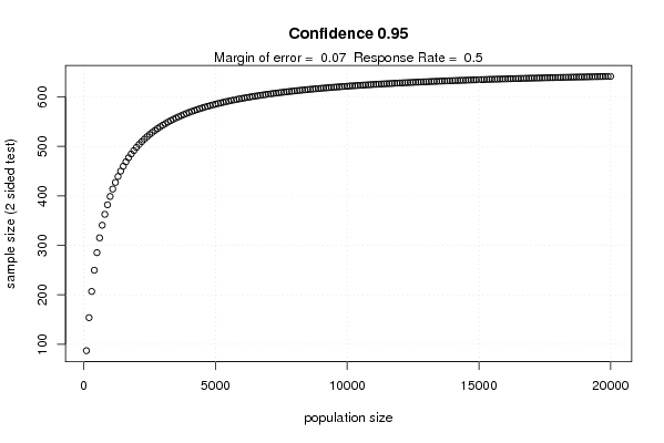
plot(ppop,npop, xlab='population size', ylab='sample size (2 sided test)', main = paste('Confidence',par3))
dumtext <- paste('Margin of error = ',par2)
dumtext <- paste(dumtext,' Response Rate = ')
dumtext <- paste(dumtext, par4)
mtext(dumtext)
grid()
dev.off()
(n <- par1 * dum / (dum + (par1-1)*par22))
(n1 <- par1 * dum1 / (dum1 + (par1-1)*par22))
load(file='createtable')
a<-table.start()
a<-table.row.start(a)
a<-table.element(a,'Minimum Sample Size',2,TRUE)
a<-table.row.end(a)
a<-table.row.start(a)
a<-table.element(a,'Population Size',header=TRUE)
a<-table.element(a,par1)
a<-table.row.end(a)
a<-table.row.start(a)
a<-table.element(a,'Margin of Error',header=TRUE)
a<-table.element(a,par2)
a<-table.row.end(a)
a<-table.row.start(a)
a<-table.element(a,'Confidence',header=TRUE)
a<-table.element(a,par3)
a<-table.row.end(a)
a<-table.row.start(a)
a<-table.element(a,'Power',header=TRUE)
a<-table.element(a,par5)
a<-table.row.end(a)
a<-table.row.start(a)
a<-table.element(a,'Response Distribution (Proportion)',header=TRUE)
a<-table.element(a,par4)
a<-table.row.end(a)
a<-table.row.start(a)
a<-table.element(a,'z(alpha/2) + z(beta)',header=TRUE)
a<-table.element(a,z)
a<-table.row.end(a)
a<-table.row.start(a)
a<-table.element(a,'z(alpha) + z(beta)',header=TRUE)
a<-table.element(a,z1)
a<-table.row.end(a)
a<-table.row.start(a)
a<-table.element(a,'Minimum Sample Size (2 sided test)',header=TRUE)
a<-table.element(a,n)
a<-table.row.end(a)
a<-table.row.start(a)
a<-table.element(a,'Minimum Sample Size (1 sided test)',header=TRUE)
a<-table.element(a,n1)
a<-table.row.end(a)
a<-table.end(a)
table.save(a,file='mytable.tab')
(n <- dum / par22)
(n1 <- dum1 / par22)
a<-table.start()
a<-table.row.start(a)
a<-table.element(a,'Minimum Sample Size (infinite population)',2,TRUE)
a<-table.row.end(a)
a<-table.row.start(a)
a<-table.element(a,'Population Size',header=TRUE)
a<-table.element(a,'infinite')
a<-table.row.end(a)
a<-table.row.start(a)
a<-table.element(a,'Margin of Error',header=TRUE)
a<-table.element(a,par2)
a<-table.row.end(a)
a<-table.row.start(a)
a<-table.element(a,'Confidence',header=TRUE)
a<-table.element(a,par3)
a<-table.row.end(a)
a<-table.row.start(a)
a<-table.element(a,'Power',header=TRUE)
a<-table.element(a,par5)
a<-table.row.end(a)
a<-table.row.start(a)
a<-table.element(a,'Response Distribution (Proportion)',header=TRUE)
a<-table.element(a,par4)
a<-table.row.end(a)
a<-table.row.start(a)
a<-table.element(a,'z(alpha/2) + z(beta)',header=TRUE)
a<-table.element(a,z)
a<-table.row.end(a)
a<-table.row.start(a)
a<-table.element(a,'z(alpha) + z(beta)',header=TRUE)
a<-table.element(a,z1)
a<-table.row.end(a)
a<-table.row.start(a)
a<-table.element(a,'Minimum Sample Size (2 sided test)',header=TRUE)
a<-table.element(a,n)
a<-table.row.end(a)
a<-table.row.start(a)
a<-table.element(a,'Minimum Sample Size (1 sided test)',header=TRUE)
a<-table.element(a,n1)
a<-table.row.end(a)
a<-table.end(a)
table.save(a,file='mytable.tab')