Free Statistics
of Irreproducible Research!
Description of Statistical Computation | |||||||||||||||||||||||||||||||||
|---|---|---|---|---|---|---|---|---|---|---|---|---|---|---|---|---|---|---|---|---|---|---|---|---|---|---|---|---|---|---|---|---|---|
| Author's title | |||||||||||||||||||||||||||||||||
| Author | *Unverified author* | ||||||||||||||||||||||||||||||||
| R Software Module | rwasp_density.wasp | ||||||||||||||||||||||||||||||||
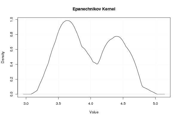
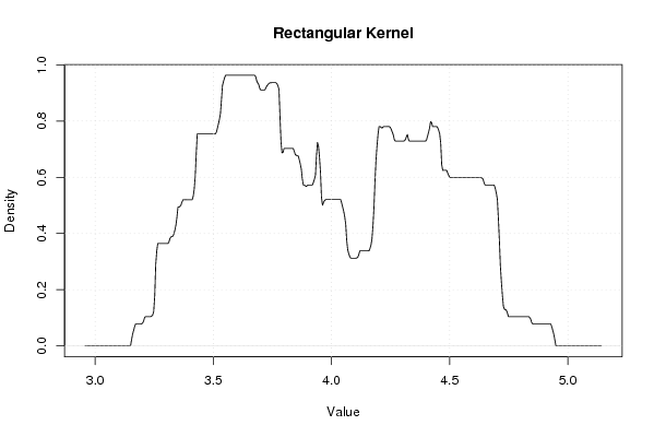
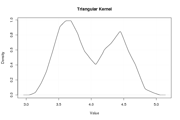
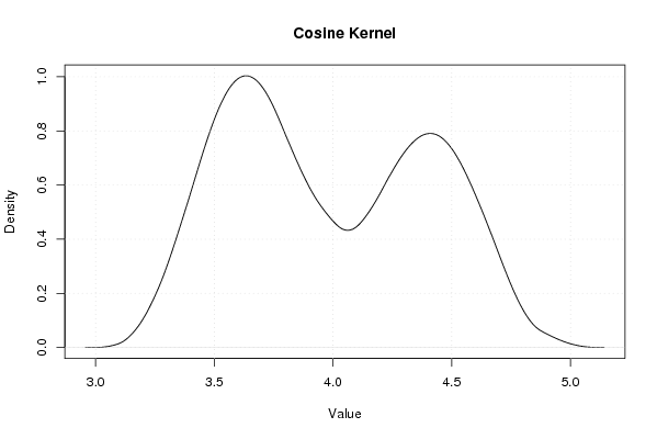
| Title produced by software | Kernel Density Estimation | ||||||||||||||||||||||||||||||||
| Date of computation | Mon, 25 Feb 2008 09:30:10 -0700 | ||||||||||||||||||||||||||||||||
| Cite this page as follows | Statistical Computations at FreeStatistics.org, Office for Research Development and Education, URL https://freestatistics.org/blog/index.php?v=date/2008/Feb/25/t12039570823rl89uwzr0h56ag.htm/, Retrieved Sat, 11 May 2024 18:39:15 +0000 | ||||||||||||||||||||||||||||||||
| Statistical Computations at FreeStatistics.org, Office for Research Development and Education, URL https://freestatistics.org/blog/index.php?pk=8960, Retrieved Sat, 11 May 2024 18:39:15 +0000 | |||||||||||||||||||||||||||||||||
| QR Codes: | |||||||||||||||||||||||||||||||||
|
| |||||||||||||||||||||||||||||||||
| Original text written by user: | |||||||||||||||||||||||||||||||||
| IsPrivate? | No (this computation is public) | ||||||||||||||||||||||||||||||||
| User-defined keywords | |||||||||||||||||||||||||||||||||
| Estimated Impact | 166 | ||||||||||||||||||||||||||||||||
Tree of Dependent Computations | |||||||||||||||||||||||||||||||||
| Family? (F = Feedback message, R = changed R code, M = changed R Module, P = changed Parameters, D = changed Data) | |||||||||||||||||||||||||||||||||
| - [Kernel Density Estimation] [Dichtheidsgrafiek...] [2008-02-25 16:30:10] [44bc6fed5801652fb7229cb9a1e49cd5] [Current] | |||||||||||||||||||||||||||||||||
| Feedback Forum | |||||||||||||||||||||||||||||||||
Post a new message | |||||||||||||||||||||||||||||||||
Dataset | |||||||||||||||||||||||||||||||||
| Dataseries X: | |||||||||||||||||||||||||||||||||
3,42 3,42 3,43 3,47 3,51 3,52 3,52 3,52 3,52 3,52 3,52 3,52 3,52 3,52 3,58 3,6 3,61 3,61 3,61 3,63 3,68 3,69 3,69 3,69 3,69 3,69 3,69 3,69 3,69 3,78 3,79 3,79 3,8 3,8 3,8 3,8 3,81 3,95 3,99 4 4,06 4,16 4,19 4,2 4,2 4,2 4,2 4,2 4,23 4,38 4,43 4,44 4,44 4,44 4,44 4,44 4,45 4,45 4,45 4,45 4,45 4,45 4,45 4,45 4,46 4,46 4,46 4,48 4,58 4,67 4,68 4,68 | |||||||||||||||||||||||||||||||||
Tables (Output of Computation) | |||||||||||||||||||||||||||||||||
| |||||||||||||||||||||||||||||||||
Figures (Output of Computation) | |||||||||||||||||||||||||||||||||
Input Parameters & R Code | |||||||||||||||||||||||||||||||||
| Parameters (Session): | |||||||||||||||||||||||||||||||||
| Parameters (R input): | |||||||||||||||||||||||||||||||||
| R code (references can be found in the software module): | |||||||||||||||||||||||||||||||||
bitmap(file='density1.png') | |||||||||||||||||||||||||||||||||