Free Statistics
of Irreproducible Research!
Description of Statistical Computation | |||||||||||||||||||||||||||||||||
|---|---|---|---|---|---|---|---|---|---|---|---|---|---|---|---|---|---|---|---|---|---|---|---|---|---|---|---|---|---|---|---|---|---|
| Author's title | |||||||||||||||||||||||||||||||||
| Author | *Unverified author* | ||||||||||||||||||||||||||||||||
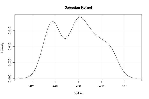
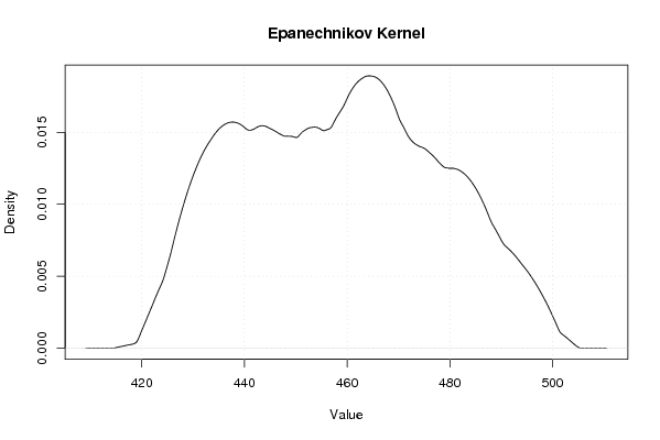
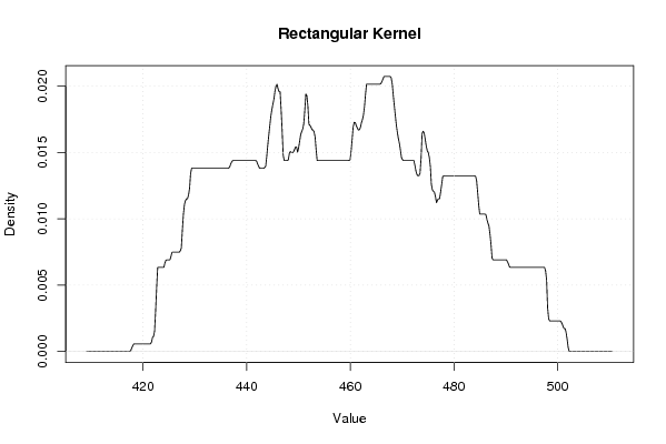
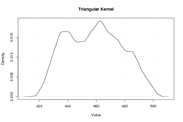
| R Software Module | rwasp_density.wasp | ||||||||||||||||||||||||||||||||
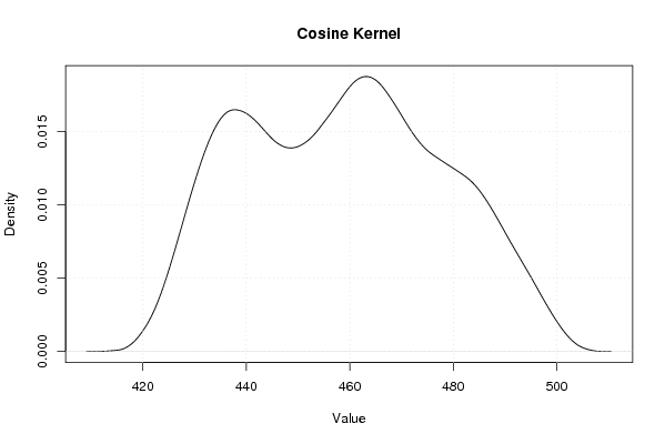
| Title produced by software | Kernel Density Estimation | ||||||||||||||||||||||||||||||||
| Date of computation | Sun, 24 Feb 2008 12:14:24 -0700 | ||||||||||||||||||||||||||||||||
| Cite this page as follows | Statistical Computations at FreeStatistics.org, Office for Research Development and Education, URL https://freestatistics.org/blog/index.php?v=date/2008/Feb/24/t1203880814pa801d5uifill6z.htm/, Retrieved Sun, 12 May 2024 05:34:44 +0000 | ||||||||||||||||||||||||||||||||
| Statistical Computations at FreeStatistics.org, Office for Research Development and Education, URL https://freestatistics.org/blog/index.php?pk=8782, Retrieved Sun, 12 May 2024 05:34:44 +0000 | |||||||||||||||||||||||||||||||||
| QR Codes: | |||||||||||||||||||||||||||||||||
|
| |||||||||||||||||||||||||||||||||
| Original text written by user: | |||||||||||||||||||||||||||||||||
| IsPrivate? | No (this computation is public) | ||||||||||||||||||||||||||||||||
| User-defined keywords | |||||||||||||||||||||||||||||||||
| Estimated Impact | 145 | ||||||||||||||||||||||||||||||||
Tree of Dependent Computations | |||||||||||||||||||||||||||||||||
| Family? (F = Feedback message, R = changed R code, M = changed R Module, P = changed Parameters, D = changed Data) | |||||||||||||||||||||||||||||||||
| - [Kernel Density Estimation] [Dichtheidsgrafiek...] [2008-02-24 19:14:24] [16094f22cd17e7ed684f81a8d68c07fe] [Current] | |||||||||||||||||||||||||||||||||
| Feedback Forum | |||||||||||||||||||||||||||||||||
Post a new message | |||||||||||||||||||||||||||||||||
Dataset | |||||||||||||||||||||||||||||||||
| Dataseries X: | |||||||||||||||||||||||||||||||||
430,00 433,87 434,55 434,55 434,55 434,55 434,71 434,71 434,71 434,71 434,73 436,34 437,55 439,58 439,65 439,76 439,76 439,76 440,06 440,13 441,18 441,14 441,14 441,19 449,06 456,46 456,79 456,87 457,25 455,93 456,00 456,22 456,22 456,58 457,61 457,61 460,43 460,43 462,18 462,37 462,59 463,19 463,48 464,30 461,41 463,35 463,35 463,35 464,27 472,28 472,36 472,56 472,56 472,56 474,15 474,59 474,97 474,99 474,99 474,99 478,34 485,70 485,75 485,85 485,84 485,85 485,84 486,00 488,79 489,71 489,71 489,71 | |||||||||||||||||||||||||||||||||
Tables (Output of Computation) | |||||||||||||||||||||||||||||||||
| |||||||||||||||||||||||||||||||||
Figures (Output of Computation) | |||||||||||||||||||||||||||||||||
Input Parameters & R Code | |||||||||||||||||||||||||||||||||
| Parameters (Session): | |||||||||||||||||||||||||||||||||
| Parameters (R input): | |||||||||||||||||||||||||||||||||
| R code (references can be found in the software module): | |||||||||||||||||||||||||||||||||
bitmap(file='density1.png') | |||||||||||||||||||||||||||||||||