Repository of Reproducible Computations

Free Statistics

of Irreproducible Research!

Author's title

Author

*The author of this computation has been verified*

R Software Module

rwasp_autocorrelation.wasp

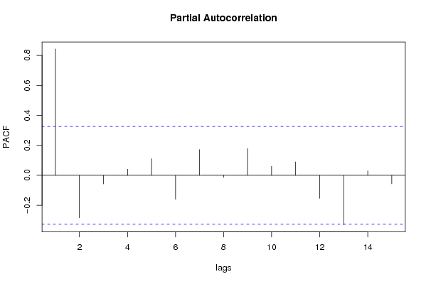
Title produced by software

(Partial) Autocorrelation Function

Date of computation

Sun, 21 Dec 2008 15:54:14 -0700

Cite this page as follows

Statistical Computations at FreeStatistics.org, Office for Research Development and Education, URL https://freestatistics.org/blog/index.php?v=date/2008/Dec/21/t1229900127qopi25jbofpfz50.htm/, Retrieved Fri, 17 May 2024 04:19:35 +0000

Statistical Computations at FreeStatistics.org, Office for Research Development and Education, URL https://freestatistics.org/blog/index.php?pk=35898, Retrieved Fri, 17 May 2024 04:19:35 +0000

QR Codes:

Paste this QR Code to cite your computation.

Original text written by user:

IsPrivate?

No (this computation is public)

User-defined keywords

Estimated Impact

183

Family? (F = Feedback message, R = changed R code, M = changed R Module, P = changed Parameters, D = changed Data)

-       [(Partial) Autocorrelation Function] [(P)ACF werkloosheid] [2008-12-21 22:54:14] [9f72e095d5529918bf5b0810c01bf6ce] [Current]
-   P     [(Partial) Autocorrelation Function] [(P)ACF werkloosheid] [2008-12-21 23:29:15] [7a4703cb85a198d9845d72899eff0288] 
-   P       [(Partial) Autocorrelation Function] [(P)ACF werklooshe...] [2008-12-22 12:23:56] [7a4703cb85a198d9845d72899eff0288] 
-   P         [(Partial) Autocorrelation Function] [(P)ACF Werklooshe...] [2008-12-22 12:31:57] [7a4703cb85a198d9845d72899eff0288] 
- RMP         [Spectral Analysis] [Spectral analysis...] [2008-12-22 12:38:27] [7a4703cb85a198d9845d72899eff0288] 
-   P           [Spectral Analysis] [Spectral Analysis...] [2008-12-22 13:08:13] [7a4703cb85a198d9845d72899eff0288] 
-   P             [Spectral Analysis] [Spectral analysis...] [2008-12-22 13:40:53] [7a4703cb85a198d9845d72899eff0288] 
-   P               [Spectral Analysis] [Spectral Analysis...] [2008-12-22 13:59:31] [7a4703cb85a198d9845d72899eff0288] 
- RMP               [ARIMA Forecasting] [] [2008-12-22 19:20:32] [b98453cac15ba1066b407e146608df68] 
- RMPD          [ARIMA Backward Selection] [ARIMA Backward Se...] [2008-12-23 13:32:19] [7a4703cb85a198d9845d72899eff0288] 
-   PD    [(Partial) Autocorrelation Function] [(P)ACF Duurzame c...] [2008-12-21 23:35:20] [7a4703cb85a198d9845d72899eff0288] 
-   PD      [(Partial) Autocorrelation Function] [(P)ACF duurzame c...] [2008-12-22 15:15:00] [7a4703cb85a198d9845d72899eff0288] 
- RMPD      [Spectral Analysis] [Spectrale analyse...] [2008-12-22 15:20:42] [7a4703cb85a198d9845d72899eff0288] 
-             [Spectral Analysis] [Spectrale analyse...] [2008-12-22 16:35:15] [7a4703cb85a198d9845d72899eff0288] 
-               [Spectral Analysis] [Spectrale analyse...] [2008-12-22 16:41:38] [7a4703cb85a198d9845d72899eff0288] 
- RM D            [ARIMA Backward Selection] [ARIMA backward se...] [2008-12-22 18:39:40] [7a4703cb85a198d9845d72899eff0288] 
-   P               [ARIMA Backward Selection] [ARIMA backward se...] [2008-12-23 11:19:18] [7a4703cb85a198d9845d72899eff0288] 
-   P               [ARIMA Backward Selection] [ARIMA Backward se...] [2008-12-23 11:24:23] [7a4703cb85a198d9845d72899eff0288] 

Feedback Forum

Post a new message

Dataseries X:

Download CSV

Histogram

Boxplots

Summary of computational transaction
Raw Input	view raw input (R code)
Raw Output	view raw output of R engine
Computing time	1 seconds
R Server	'George Udny Yule' @ 72.249.76.132

\begin{tabular}{lllllllll}
\hline
Summary of computational transaction \tabularnewline
Raw Input & view raw input (R code)  \tabularnewline
Raw Output & view raw output of R engine  \tabularnewline
Computing time & 1 seconds \tabularnewline
R Server & 'George Udny Yule' @ 72.249.76.132 \tabularnewline
\hline
\end{tabular}
%Source: https://freestatistics.org/blog/index.php?pk=35898&T=0

[TABLE]
[ROW][C]Summary of computational transaction[/C][/ROW]
[ROW][C]Raw Input[/C][C]view raw input (R code) [/C][/ROW]
[ROW][C]Raw Output[/C][C]view raw output of R engine [/C][/ROW]
[ROW][C]Computing time[/C][C]1 seconds[/C][/ROW]
[ROW][C]R Server[/C][C]'George Udny Yule' @ 72.249.76.132[/C][/ROW]
[/TABLE]
Source: https://freestatistics.org/blog/index.php?pk=35898&T=0

Globally Unique Identifier (entire table): ba.freestatistics.org/blog/index.php?pk=35898&T=0

As an alternative you can also use a QR Code:

The GUIDs for individual cells are displayed in the table below:

Summary of computational transaction
Raw Input	view raw input (R code)
Raw Output	view raw output of R engine
Computing time	1 seconds
R Server	'George Udny Yule' @ 72.249.76.132

Autocorrelation Function
Time lag k	ACF(k)	T-STAT	P-value
1	0.84321	5.0593	6e-06
2	0.62909	3.7745	0.000289
3	0.426632	2.5598	0.007409
4	0.278088	1.6685	0.051944
5	0.206877	1.2413	0.111268
6	0.134235	0.8054	0.212935
7	0.114923	0.6895	0.247452
8	0.111119	0.6667	0.254602
9	0.153679	0.9221	0.181315
10	0.223948	1.3437	0.093729
11	0.284774	1.7086	0.048063
12	0.29156	1.7494	0.044375
13	0.163773	0.9826	0.166172
14	0.020785	0.1247	0.450724
15	-0.109097	-0.6546	0.258449

\begin{tabular}{lllllllll}
\hline
Autocorrelation Function \tabularnewline
Time lag k & ACF(k) & T-STAT & P-value \tabularnewline
1 & 0.84321 & 5.0593 & 6e-06 \tabularnewline
2 & 0.62909 & 3.7745 & 0.000289 \tabularnewline
3 & 0.426632 & 2.5598 & 0.007409 \tabularnewline
4 & 0.278088 & 1.6685 & 0.051944 \tabularnewline
5 & 0.206877 & 1.2413 & 0.111268 \tabularnewline
6 & 0.134235 & 0.8054 & 0.212935 \tabularnewline
7 & 0.114923 & 0.6895 & 0.247452 \tabularnewline
8 & 0.111119 & 0.6667 & 0.254602 \tabularnewline
9 & 0.153679 & 0.9221 & 0.181315 \tabularnewline
10 & 0.223948 & 1.3437 & 0.093729 \tabularnewline
11 & 0.284774 & 1.7086 & 0.048063 \tabularnewline
12 & 0.29156 & 1.7494 & 0.044375 \tabularnewline
13 & 0.163773 & 0.9826 & 0.166172 \tabularnewline
14 & 0.020785 & 0.1247 & 0.450724 \tabularnewline
15 & -0.109097 & -0.6546 & 0.258449 \tabularnewline
\hline
\end{tabular}
%Source: https://freestatistics.org/blog/index.php?pk=35898&T=1

[TABLE]
[ROW][C]Autocorrelation Function[/C][/ROW]
[ROW][C]Time lag k[/C][C]ACF(k)[/C][C]T-STAT[/C][C]P-value[/C][/ROW]
[ROW][C]1[/C][C]0.84321[/C][C]5.0593[/C][C]6e-06[/C][/ROW]
[ROW][C]2[/C][C]0.62909[/C][C]3.7745[/C][C]0.000289[/C][/ROW]
[ROW][C]3[/C][C]0.426632[/C][C]2.5598[/C][C]0.007409[/C][/ROW]
[ROW][C]4[/C][C]0.278088[/C][C]1.6685[/C][C]0.051944[/C][/ROW]
[ROW][C]5[/C][C]0.206877[/C][C]1.2413[/C][C]0.111268[/C][/ROW]
[ROW][C]6[/C][C]0.134235[/C][C]0.8054[/C][C]0.212935[/C][/ROW]
[ROW][C]7[/C][C]0.114923[/C][C]0.6895[/C][C]0.247452[/C][/ROW]
[ROW][C]8[/C][C]0.111119[/C][C]0.6667[/C][C]0.254602[/C][/ROW]
[ROW][C]9[/C][C]0.153679[/C][C]0.9221[/C][C]0.181315[/C][/ROW]
[ROW][C]10[/C][C]0.223948[/C][C]1.3437[/C][C]0.093729[/C][/ROW]
[ROW][C]11[/C][C]0.284774[/C][C]1.7086[/C][C]0.048063[/C][/ROW]
[ROW][C]12[/C][C]0.29156[/C][C]1.7494[/C][C]0.044375[/C][/ROW]
[ROW][C]13[/C][C]0.163773[/C][C]0.9826[/C][C]0.166172[/C][/ROW]
[ROW][C]14[/C][C]0.020785[/C][C]0.1247[/C][C]0.450724[/C][/ROW]
[ROW][C]15[/C][C]-0.109097[/C][C]-0.6546[/C][C]0.258449[/C][/ROW]
[/TABLE]
Source: https://freestatistics.org/blog/index.php?pk=35898&T=1

Globally Unique Identifier (entire table): ba.freestatistics.org/blog/index.php?pk=35898&T=1

As an alternative you can also use a QR Code:

The GUIDs for individual cells are displayed in the table below:

Autocorrelation Function
Time lag k	ACF(k)	T-STAT	P-value
1	0.84321	5.0593	6e-06
2	0.62909	3.7745	0.000289
3	0.426632	2.5598	0.007409
4	0.278088	1.6685	0.051944
5	0.206877	1.2413	0.111268
6	0.134235	0.8054	0.212935
7	0.114923	0.6895	0.247452
8	0.111119	0.6667	0.254602
9	0.153679	0.9221	0.181315
10	0.223948	1.3437	0.093729
11	0.284774	1.7086	0.048063
12	0.29156	1.7494	0.044375
13	0.163773	0.9826	0.166172
14	0.020785	0.1247	0.450724
15	-0.109097	-0.6546	0.258449

Partial Autocorrelation Function
Time lag k	PACF(k)	T-STAT	P-value
1	0.84321	5.0593	6e-06
2	-0.28344	-1.7006	0.048818
3	-0.0571	-0.3426	0.366945
4	0.04103	0.2462	0.403471
5	0.110784	0.6647	0.255238
6	-0.159391	-0.9563	0.172638
7	0.171267	1.0276	0.155496
8	-0.012915	-0.0775	0.469331
9	0.178944	1.0737	0.145059
10	0.060098	0.3606	0.360257
11	0.089268	0.5356	0.297762
12	-0.153197	-0.9192	0.182059
13	-0.330133	-1.9808	0.027647
14	0.030186	0.1811	0.428647
15	-0.056804	-0.3408	0.367608

\begin{tabular}{lllllllll}
\hline
Partial Autocorrelation Function \tabularnewline
Time lag k & PACF(k) & T-STAT & P-value \tabularnewline
1 & 0.84321 & 5.0593 & 6e-06 \tabularnewline
2 & -0.28344 & -1.7006 & 0.048818 \tabularnewline
3 & -0.0571 & -0.3426 & 0.366945 \tabularnewline
4 & 0.04103 & 0.2462 & 0.403471 \tabularnewline
5 & 0.110784 & 0.6647 & 0.255238 \tabularnewline
6 & -0.159391 & -0.9563 & 0.172638 \tabularnewline
7 & 0.171267 & 1.0276 & 0.155496 \tabularnewline
8 & -0.012915 & -0.0775 & 0.469331 \tabularnewline
9 & 0.178944 & 1.0737 & 0.145059 \tabularnewline
10 & 0.060098 & 0.3606 & 0.360257 \tabularnewline
11 & 0.089268 & 0.5356 & 0.297762 \tabularnewline
12 & -0.153197 & -0.9192 & 0.182059 \tabularnewline
13 & -0.330133 & -1.9808 & 0.027647 \tabularnewline
14 & 0.030186 & 0.1811 & 0.428647 \tabularnewline
15 & -0.056804 & -0.3408 & 0.367608 \tabularnewline
\hline
\end{tabular}
%Source: https://freestatistics.org/blog/index.php?pk=35898&T=2

[TABLE]
[ROW][C]Partial Autocorrelation Function[/C][/ROW]
[ROW][C]Time lag k[/C][C]PACF(k)[/C][C]T-STAT[/C][C]P-value[/C][/ROW]
[ROW][C]1[/C][C]0.84321[/C][C]5.0593[/C][C]6e-06[/C][/ROW]
[ROW][C]2[/C][C]-0.28344[/C][C]-1.7006[/C][C]0.048818[/C][/ROW]
[ROW][C]3[/C][C]-0.0571[/C][C]-0.3426[/C][C]0.366945[/C][/ROW]
[ROW][C]4[/C][C]0.04103[/C][C]0.2462[/C][C]0.403471[/C][/ROW]
[ROW][C]5[/C][C]0.110784[/C][C]0.6647[/C][C]0.255238[/C][/ROW]
[ROW][C]6[/C][C]-0.159391[/C][C]-0.9563[/C][C]0.172638[/C][/ROW]
[ROW][C]7[/C][C]0.171267[/C][C]1.0276[/C][C]0.155496[/C][/ROW]
[ROW][C]8[/C][C]-0.012915[/C][C]-0.0775[/C][C]0.469331[/C][/ROW]
[ROW][C]9[/C][C]0.178944[/C][C]1.0737[/C][C]0.145059[/C][/ROW]
[ROW][C]10[/C][C]0.060098[/C][C]0.3606[/C][C]0.360257[/C][/ROW]
[ROW][C]11[/C][C]0.089268[/C][C]0.5356[/C][C]0.297762[/C][/ROW]
[ROW][C]12[/C][C]-0.153197[/C][C]-0.9192[/C][C]0.182059[/C][/ROW]
[ROW][C]13[/C][C]-0.330133[/C][C]-1.9808[/C][C]0.027647[/C][/ROW]
[ROW][C]14[/C][C]0.030186[/C][C]0.1811[/C][C]0.428647[/C][/ROW]
[ROW][C]15[/C][C]-0.056804[/C][C]-0.3408[/C][C]0.367608[/C][/ROW]
[/TABLE]
Source: https://freestatistics.org/blog/index.php?pk=35898&T=2

Globally Unique Identifier (entire table): ba.freestatistics.org/blog/index.php?pk=35898&T=2

As an alternative you can also use a QR Code:

The GUIDs for individual cells are displayed in the table below:

Partial Autocorrelation Function
Time lag k	PACF(k)	T-STAT	P-value
1	0.84321	5.0593	6e-06
2	-0.28344	-1.7006	0.048818
3	-0.0571	-0.3426	0.366945
4	0.04103	0.2462	0.403471
5	0.110784	0.6647	0.255238
6	-0.159391	-0.9563	0.172638
7	0.171267	1.0276	0.155496
8	-0.012915	-0.0775	0.469331
9	0.178944	1.0737	0.145059
10	0.060098	0.3606	0.360257
11	0.089268	0.5356	0.297762
12	-0.153197	-0.9192	0.182059
13	-0.330133	-1.9808	0.027647
14	0.030186	0.1811	0.428647
15	-0.056804	-0.3408	0.367608

Figure 1

PNG link

Postscript link

PDF link

Figure 2

PNG link

Postscript link

PDF link

Parameters (Session):

par1 = Default ; par2 = 1 ; par3 = 0 ; par4 = 0 ; par5 = 12 ;

Parameters (R input):

par1 = Default ; par2 = 1 ; par3 = 0 ; par4 = 0 ; par5 = 12 ;

R code (references can be found in the software module):

if (par1 == 'Default') {
par1 = 10*log10(length(x))
} else {
par1 <- as.numeric(par1)
}
par2 <- as.numeric(par2)
par3 <- as.numeric(par3)
par4 <- as.numeric(par4)
par5 <- as.numeric(par5)
if (par2 == 0) {
x <- log(x)
} else {
x <- (x ^ par2 - 1) / par2
}
if (par3 > 0) x <- diff(x,lag=1,difference=par3)
if (par4 > 0) x <- diff(x,lag=par5,difference=par4)
bitmap(file='pic1.png')
racf <- acf(x,par1,main='Autocorrelation',xlab='lags',ylab='ACF')
dev.off()
bitmap(file='pic2.png')
rpacf <- pacf(x,par1,main='Partial Autocorrelation',xlab='lags',ylab='PACF')
dev.off()
(myacf <- c(racf$acf))
(mypacf <- c(rpacf$acf))
lengthx <- length(x)
sqrtn <- sqrt(lengthx)
load(file='createtable')
a<-table.start()
a<-table.row.start(a)
a<-table.element(a,'Autocorrelation Function',4,TRUE)
a<-table.row.end(a)
a<-table.row.start(a)
a<-table.element(a,'Time lag k',header=TRUE)
a<-table.element(a,hyperlink('basics.htm','ACF(k)','click here for more information about the Autocorrelation Function'),header=TRUE)
a<-table.element(a,'T-STAT',header=TRUE)
a<-table.element(a,'P-value',header=TRUE)
a<-table.row.end(a)
for (i in 2:(par1+1)) {
a<-table.row.start(a)
a<-table.element(a,i-1,header=TRUE)
a<-table.element(a,round(myacf[i],6))
mytstat <- myacf[i]*sqrtn
a<-table.element(a,round(mytstat,4))
a<-table.element(a,round(1-pt(abs(mytstat),lengthx),6))
a<-table.row.end(a)
}
a<-table.end(a)
table.save(a,file='mytable.tab')
a<-table.start()
a<-table.row.start(a)
a<-table.element(a,'Partial Autocorrelation Function',4,TRUE)
a<-table.row.end(a)
a<-table.row.start(a)
a<-table.element(a,'Time lag k',header=TRUE)
a<-table.element(a,hyperlink('basics.htm','PACF(k)','click here for more information about the Partial Autocorrelation Function'),header=TRUE)
a<-table.element(a,'T-STAT',header=TRUE)
a<-table.element(a,'P-value',header=TRUE)
a<-table.row.end(a)
for (i in 1:par1) {
a<-table.row.start(a)
a<-table.element(a,i,header=TRUE)
a<-table.element(a,round(mypacf[i],6))
mytstat <- mypacf[i]*sqrtn
a<-table.element(a,round(mytstat,4))
a<-table.element(a,round(1-pt(abs(mytstat),lengthx),6))
a<-table.row.end(a)
}
a<-table.end(a)
table.save(a,file='mytable1.tab')

Free Statistics

Description of Statistical Computation

Tree of Dependent Computations

Dataset

Tables (Output of Computation)

Figures (Output of Computation)

Input Parameters & R Code