Repository of Reproducible Computations

Free Statistics

of Irreproducible Research!

Author's title

Author

*The author of this computation has been verified*

R Software Module

rwasp_autocorrelation.wasp

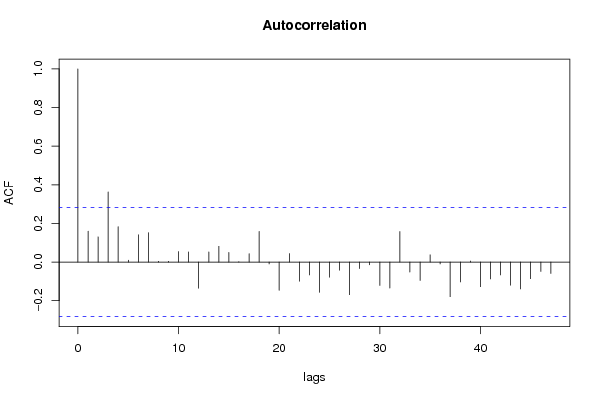
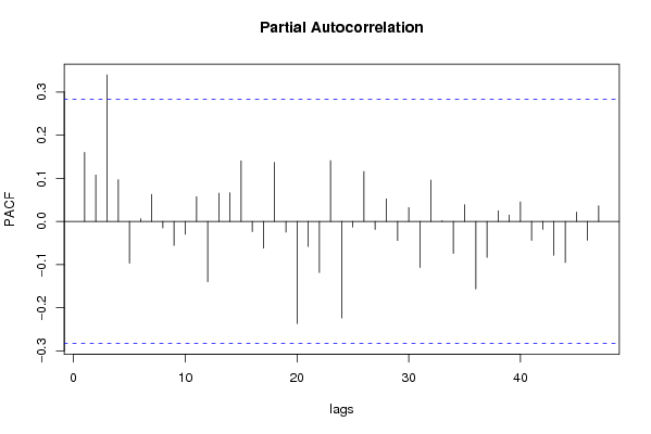
Title produced by software

(Partial) Autocorrelation Function

Date of computation

Sun, 14 Dec 2008 08:50:28 -0700

Cite this page as follows

Statistical Computations at FreeStatistics.org, Office for Research Development and Education, URL https://freestatistics.org/blog/index.php?v=date/2008/Dec/14/t1229269861ejla549ynty14ne.htm/, Retrieved Fri, 17 May 2024 07:01:27 +0000

Statistical Computations at FreeStatistics.org, Office for Research Development and Education, URL https://freestatistics.org/blog/index.php?pk=33442, Retrieved Fri, 17 May 2024 07:01:27 +0000

QR Codes:

Paste this QR Code to cite your computation.

Original text written by user:

IsPrivate?

No (this computation is public)

User-defined keywords

Estimated Impact

177

Family? (F = Feedback message, R = changed R code, M = changed R Module, P = changed Parameters, D = changed Data)

F     [Variance Reduction Matrix] [workshop] [2008-12-14 15:44:19] [3a9fc6d5b5e0e816787b7dbace57e7cd]
F RMP   [Spectral Analysis] [workshop] [2008-12-14 15:45:47] [3a9fc6d5b5e0e816787b7dbace57e7cd]
F   P     [Spectral Analysis] [workshop] [2008-12-14 15:47:26] [3a9fc6d5b5e0e816787b7dbace57e7cd]
F RMP       [Standard Deviation-Mean Plot] [workshop] [2008-12-14 15:48:50] [3a9fc6d5b5e0e816787b7dbace57e7cd]
F RMP           [(Partial) Autocorrelation Function] [workshop] [2008-12-14 15:50:28] [821c4b3d195be8e737cf8c9dc649d3cf] [Current]
F RMP             [ARIMA Backward Selection] [workshop] [2008-12-14 15:55:32] [3a9fc6d5b5e0e816787b7dbace57e7cd] 
F RMP               [ARIMA Forecasting] [workshop] [2008-12-14 15:58:35] [3a9fc6d5b5e0e816787b7dbace57e7cd] 

Feedback Forum

2008-12-24 07:29:54 [Gert-Jan Geudens] [reply] 
Correct we hebben hier inderdaad een stationaire reeks bekomen. Voor meer uitleg verwijzen we graag naar de vorige workshops waar dit reeds zeer uitvoerig is besproken. Het was zeer goed om eerst de gekozen parameters voor de ARIMA Forecast kort te verantwoorden.

Post a new message

Dataseries X:

Download CSV

Histogram

Boxplots

Summary of computational transaction
Raw Input	view raw input (R code)
Raw Output	view raw output of R engine
Computing time	3 seconds
R Server	'Herman Ole Andreas Wold' @ 193.190.124.10:1001

\begin{tabular}{lllllllll}
\hline
Summary of computational transaction \tabularnewline
Raw Input & view raw input (R code)  \tabularnewline
Raw Output & view raw output of R engine  \tabularnewline
Computing time & 3 seconds \tabularnewline
R Server & 'Herman Ole Andreas Wold' @ 193.190.124.10:1001 \tabularnewline
\hline
\end{tabular}
%Source: https://freestatistics.org/blog/index.php?pk=33442&T=0

[TABLE]
[ROW][C]Summary of computational transaction[/C][/ROW]
[ROW][C]Raw Input[/C][C]view raw input (R code) [/C][/ROW]
[ROW][C]Raw Output[/C][C]view raw output of R engine [/C][/ROW]
[ROW][C]Computing time[/C][C]3 seconds[/C][/ROW]
[ROW][C]R Server[/C][C]'Herman Ole Andreas Wold' @ 193.190.124.10:1001[/C][/ROW]
[/TABLE]
Source: https://freestatistics.org/blog/index.php?pk=33442&T=0

Globally Unique Identifier (entire table): ba.freestatistics.org/blog/index.php?pk=33442&T=0

As an alternative you can also use a QR Code:

The GUIDs for individual cells are displayed in the table below:

Summary of computational transaction
Raw Input	view raw input (R code)
Raw Output	view raw output of R engine
Computing time	3 seconds
R Server	'Herman Ole Andreas Wold' @ 193.190.124.10:1001

Autocorrelation Function
Time lag k	ACF(k)	T-STAT	P-value
1	0.159946	1.1081	0.136661
2	0.130298	0.9027	0.185589
3	0.362996	2.5149	0.007655
4	0.18309	1.2685	0.105371
5	0.009554	0.0662	0.473749
6	0.141305	0.979	0.166246
7	0.151799	1.0517	0.149103
8	0.004048	0.028	0.488871
9	0.003631	0.0252	0.490018
10	0.05395	0.3738	0.355107
11	0.052199	0.3616	0.359602
12	-0.135809	-0.9409	0.175731
13	0.052633	0.3647	0.358486
14	0.081161	0.5623	0.288263
15	0.049415	0.3424	0.366789
16	0.002012	0.0139	0.494469
17	0.043251	0.2997	0.382868
18	0.158709	1.0996	0.138502
19	-0.009958	-0.069	0.472641
20	-0.146455	-1.0147	0.157676
21	0.04359	0.302	0.381978
22	-0.099498	-0.6893	0.246964
23	-0.06657	-0.4612	0.323365
24	-0.156666	-1.0854	0.14158
25	-0.078424	-0.5433	0.294705
26	-0.042342	-0.2934	0.385259
27	-0.168987	-1.1708	0.123734
28	-0.03388	-0.2347	0.40771
29	-0.014274	-0.0989	0.460818
30	-0.121193	-0.8397	0.202633
31	-0.134831	-0.9341	0.177455
32	0.157635	1.0921	0.140115
33	-0.051704	-0.3582	0.360876
34	-0.095595	-0.6623	0.255473
35	0.037684	0.2611	0.397572
36	-0.010112	-0.0701	0.472219
37	-0.179251	-1.2419	0.110156
38	-0.103148	-0.7146	0.23915
39	0.005121	0.0355	0.485922
40	-0.127875	-0.8859	0.190033
41	-0.087277	-0.6047	0.274123
42	-0.066588	-0.4613	0.32332
43	-0.12023	-0.833	0.204492
44	-0.139517	-0.9666	0.169294
45	-0.086069	-0.5963	0.276887
46	-0.048916	-0.3389	0.368081
47	-0.058861	-0.4078	0.342618
48	NA	NA	NA
49	NA	NA	NA
50	NA	NA	NA
51	NA	NA	NA
52	NA	NA	NA
53	NA	NA	NA
54	NA	NA	NA
55	NA	NA	NA
56	NA	NA	NA
57	NA	NA	NA
58	NA	NA	NA
59	NA	NA	NA
60	NA	NA	NA

\begin{tabular}{lllllllll}
\hline
Autocorrelation Function \tabularnewline
Time lag k & ACF(k) & T-STAT & P-value \tabularnewline
1 & 0.159946 & 1.1081 & 0.136661 \tabularnewline
2 & 0.130298 & 0.9027 & 0.185589 \tabularnewline
3 & 0.362996 & 2.5149 & 0.007655 \tabularnewline
4 & 0.18309 & 1.2685 & 0.105371 \tabularnewline
5 & 0.009554 & 0.0662 & 0.473749 \tabularnewline
6 & 0.141305 & 0.979 & 0.166246 \tabularnewline
7 & 0.151799 & 1.0517 & 0.149103 \tabularnewline
8 & 0.004048 & 0.028 & 0.488871 \tabularnewline
9 & 0.003631 & 0.0252 & 0.490018 \tabularnewline
10 & 0.05395 & 0.3738 & 0.355107 \tabularnewline
11 & 0.052199 & 0.3616 & 0.359602 \tabularnewline
12 & -0.135809 & -0.9409 & 0.175731 \tabularnewline
13 & 0.052633 & 0.3647 & 0.358486 \tabularnewline
14 & 0.081161 & 0.5623 & 0.288263 \tabularnewline
15 & 0.049415 & 0.3424 & 0.366789 \tabularnewline
16 & 0.002012 & 0.0139 & 0.494469 \tabularnewline
17 & 0.043251 & 0.2997 & 0.382868 \tabularnewline
18 & 0.158709 & 1.0996 & 0.138502 \tabularnewline
19 & -0.009958 & -0.069 & 0.472641 \tabularnewline
20 & -0.146455 & -1.0147 & 0.157676 \tabularnewline
21 & 0.04359 & 0.302 & 0.381978 \tabularnewline
22 & -0.099498 & -0.6893 & 0.246964 \tabularnewline
23 & -0.06657 & -0.4612 & 0.323365 \tabularnewline
24 & -0.156666 & -1.0854 & 0.14158 \tabularnewline
25 & -0.078424 & -0.5433 & 0.294705 \tabularnewline
26 & -0.042342 & -0.2934 & 0.385259 \tabularnewline
27 & -0.168987 & -1.1708 & 0.123734 \tabularnewline
28 & -0.03388 & -0.2347 & 0.40771 \tabularnewline
29 & -0.014274 & -0.0989 & 0.460818 \tabularnewline
30 & -0.121193 & -0.8397 & 0.202633 \tabularnewline
31 & -0.134831 & -0.9341 & 0.177455 \tabularnewline
32 & 0.157635 & 1.0921 & 0.140115 \tabularnewline
33 & -0.051704 & -0.3582 & 0.360876 \tabularnewline
34 & -0.095595 & -0.6623 & 0.255473 \tabularnewline
35 & 0.037684 & 0.2611 & 0.397572 \tabularnewline
36 & -0.010112 & -0.0701 & 0.472219 \tabularnewline
37 & -0.179251 & -1.2419 & 0.110156 \tabularnewline
38 & -0.103148 & -0.7146 & 0.23915 \tabularnewline
39 & 0.005121 & 0.0355 & 0.485922 \tabularnewline
40 & -0.127875 & -0.8859 & 0.190033 \tabularnewline
41 & -0.087277 & -0.6047 & 0.274123 \tabularnewline
42 & -0.066588 & -0.4613 & 0.32332 \tabularnewline
43 & -0.12023 & -0.833 & 0.204492 \tabularnewline
44 & -0.139517 & -0.9666 & 0.169294 \tabularnewline
45 & -0.086069 & -0.5963 & 0.276887 \tabularnewline
46 & -0.048916 & -0.3389 & 0.368081 \tabularnewline
47 & -0.058861 & -0.4078 & 0.342618 \tabularnewline
48 & NA & NA & NA \tabularnewline
49 & NA & NA & NA \tabularnewline
50 & NA & NA & NA \tabularnewline
51 & NA & NA & NA \tabularnewline
52 & NA & NA & NA \tabularnewline
53 & NA & NA & NA \tabularnewline
54 & NA & NA & NA \tabularnewline
55 & NA & NA & NA \tabularnewline
56 & NA & NA & NA \tabularnewline
57 & NA & NA & NA \tabularnewline
58 & NA & NA & NA \tabularnewline
59 & NA & NA & NA \tabularnewline
60 & NA & NA & NA \tabularnewline
\hline
\end{tabular}
%Source: https://freestatistics.org/blog/index.php?pk=33442&T=1

[TABLE]
[ROW][C]Autocorrelation Function[/C][/ROW]
[ROW][C]Time lag k[/C][C]ACF(k)[/C][C]T-STAT[/C][C]P-value[/C][/ROW]
[ROW][C]1[/C][C]0.159946[/C][C]1.1081[/C][C]0.136661[/C][/ROW]
[ROW][C]2[/C][C]0.130298[/C][C]0.9027[/C][C]0.185589[/C][/ROW]
[ROW][C]3[/C][C]0.362996[/C][C]2.5149[/C][C]0.007655[/C][/ROW]
[ROW][C]4[/C][C]0.18309[/C][C]1.2685[/C][C]0.105371[/C][/ROW]
[ROW][C]5[/C][C]0.009554[/C][C]0.0662[/C][C]0.473749[/C][/ROW]
[ROW][C]6[/C][C]0.141305[/C][C]0.979[/C][C]0.166246[/C][/ROW]
[ROW][C]7[/C][C]0.151799[/C][C]1.0517[/C][C]0.149103[/C][/ROW]
[ROW][C]8[/C][C]0.004048[/C][C]0.028[/C][C]0.488871[/C][/ROW]
[ROW][C]9[/C][C]0.003631[/C][C]0.0252[/C][C]0.490018[/C][/ROW]
[ROW][C]10[/C][C]0.05395[/C][C]0.3738[/C][C]0.355107[/C][/ROW]
[ROW][C]11[/C][C]0.052199[/C][C]0.3616[/C][C]0.359602[/C][/ROW]
[ROW][C]12[/C][C]-0.135809[/C][C]-0.9409[/C][C]0.175731[/C][/ROW]
[ROW][C]13[/C][C]0.052633[/C][C]0.3647[/C][C]0.358486[/C][/ROW]
[ROW][C]14[/C][C]0.081161[/C][C]0.5623[/C][C]0.288263[/C][/ROW]
[ROW][C]15[/C][C]0.049415[/C][C]0.3424[/C][C]0.366789[/C][/ROW]
[ROW][C]16[/C][C]0.002012[/C][C]0.0139[/C][C]0.494469[/C][/ROW]
[ROW][C]17[/C][C]0.043251[/C][C]0.2997[/C][C]0.382868[/C][/ROW]
[ROW][C]18[/C][C]0.158709[/C][C]1.0996[/C][C]0.138502[/C][/ROW]
[ROW][C]19[/C][C]-0.009958[/C][C]-0.069[/C][C]0.472641[/C][/ROW]
[ROW][C]20[/C][C]-0.146455[/C][C]-1.0147[/C][C]0.157676[/C][/ROW]
[ROW][C]21[/C][C]0.04359[/C][C]0.302[/C][C]0.381978[/C][/ROW]
[ROW][C]22[/C][C]-0.099498[/C][C]-0.6893[/C][C]0.246964[/C][/ROW]
[ROW][C]23[/C][C]-0.06657[/C][C]-0.4612[/C][C]0.323365[/C][/ROW]
[ROW][C]24[/C][C]-0.156666[/C][C]-1.0854[/C][C]0.14158[/C][/ROW]
[ROW][C]25[/C][C]-0.078424[/C][C]-0.5433[/C][C]0.294705[/C][/ROW]
[ROW][C]26[/C][C]-0.042342[/C][C]-0.2934[/C][C]0.385259[/C][/ROW]
[ROW][C]27[/C][C]-0.168987[/C][C]-1.1708[/C][C]0.123734[/C][/ROW]
[ROW][C]28[/C][C]-0.03388[/C][C]-0.2347[/C][C]0.40771[/C][/ROW]
[ROW][C]29[/C][C]-0.014274[/C][C]-0.0989[/C][C]0.460818[/C][/ROW]
[ROW][C]30[/C][C]-0.121193[/C][C]-0.8397[/C][C]0.202633[/C][/ROW]
[ROW][C]31[/C][C]-0.134831[/C][C]-0.9341[/C][C]0.177455[/C][/ROW]
[ROW][C]32[/C][C]0.157635[/C][C]1.0921[/C][C]0.140115[/C][/ROW]
[ROW][C]33[/C][C]-0.051704[/C][C]-0.3582[/C][C]0.360876[/C][/ROW]
[ROW][C]34[/C][C]-0.095595[/C][C]-0.6623[/C][C]0.255473[/C][/ROW]
[ROW][C]35[/C][C]0.037684[/C][C]0.2611[/C][C]0.397572[/C][/ROW]
[ROW][C]36[/C][C]-0.010112[/C][C]-0.0701[/C][C]0.472219[/C][/ROW]
[ROW][C]37[/C][C]-0.179251[/C][C]-1.2419[/C][C]0.110156[/C][/ROW]
[ROW][C]38[/C][C]-0.103148[/C][C]-0.7146[/C][C]0.23915[/C][/ROW]
[ROW][C]39[/C][C]0.005121[/C][C]0.0355[/C][C]0.485922[/C][/ROW]
[ROW][C]40[/C][C]-0.127875[/C][C]-0.8859[/C][C]0.190033[/C][/ROW]
[ROW][C]41[/C][C]-0.087277[/C][C]-0.6047[/C][C]0.274123[/C][/ROW]
[ROW][C]42[/C][C]-0.066588[/C][C]-0.4613[/C][C]0.32332[/C][/ROW]
[ROW][C]43[/C][C]-0.12023[/C][C]-0.833[/C][C]0.204492[/C][/ROW]
[ROW][C]44[/C][C]-0.139517[/C][C]-0.9666[/C][C]0.169294[/C][/ROW]
[ROW][C]45[/C][C]-0.086069[/C][C]-0.5963[/C][C]0.276887[/C][/ROW]
[ROW][C]46[/C][C]-0.048916[/C][C]-0.3389[/C][C]0.368081[/C][/ROW]
[ROW][C]47[/C][C]-0.058861[/C][C]-0.4078[/C][C]0.342618[/C][/ROW]
[ROW][C]48[/C][C]NA[/C][C]NA[/C][C]NA[/C][/ROW]
[ROW][C]49[/C][C]NA[/C][C]NA[/C][C]NA[/C][/ROW]
[ROW][C]50[/C][C]NA[/C][C]NA[/C][C]NA[/C][/ROW]
[ROW][C]51[/C][C]NA[/C][C]NA[/C][C]NA[/C][/ROW]
[ROW][C]52[/C][C]NA[/C][C]NA[/C][C]NA[/C][/ROW]
[ROW][C]53[/C][C]NA[/C][C]NA[/C][C]NA[/C][/ROW]
[ROW][C]54[/C][C]NA[/C][C]NA[/C][C]NA[/C][/ROW]
[ROW][C]55[/C][C]NA[/C][C]NA[/C][C]NA[/C][/ROW]
[ROW][C]56[/C][C]NA[/C][C]NA[/C][C]NA[/C][/ROW]
[ROW][C]57[/C][C]NA[/C][C]NA[/C][C]NA[/C][/ROW]
[ROW][C]58[/C][C]NA[/C][C]NA[/C][C]NA[/C][/ROW]
[ROW][C]59[/C][C]NA[/C][C]NA[/C][C]NA[/C][/ROW]
[ROW][C]60[/C][C]NA[/C][C]NA[/C][C]NA[/C][/ROW]
[/TABLE]
Source: https://freestatistics.org/blog/index.php?pk=33442&T=1

Globally Unique Identifier (entire table): ba.freestatistics.org/blog/index.php?pk=33442&T=1

As an alternative you can also use a QR Code:

The GUIDs for individual cells are displayed in the table below:

Autocorrelation Function
Time lag k	ACF(k)	T-STAT	P-value
1	0.159946	1.1081	0.136661
2	0.130298	0.9027	0.185589
3	0.362996	2.5149	0.007655
4	0.18309	1.2685	0.105371
5	0.009554	0.0662	0.473749
6	0.141305	0.979	0.166246
7	0.151799	1.0517	0.149103
8	0.004048	0.028	0.488871
9	0.003631	0.0252	0.490018
10	0.05395	0.3738	0.355107
11	0.052199	0.3616	0.359602
12	-0.135809	-0.9409	0.175731
13	0.052633	0.3647	0.358486
14	0.081161	0.5623	0.288263
15	0.049415	0.3424	0.366789
16	0.002012	0.0139	0.494469
17	0.043251	0.2997	0.382868
18	0.158709	1.0996	0.138502
19	-0.009958	-0.069	0.472641
20	-0.146455	-1.0147	0.157676
21	0.04359	0.302	0.381978
22	-0.099498	-0.6893	0.246964
23	-0.06657	-0.4612	0.323365
24	-0.156666	-1.0854	0.14158
25	-0.078424	-0.5433	0.294705
26	-0.042342	-0.2934	0.385259
27	-0.168987	-1.1708	0.123734
28	-0.03388	-0.2347	0.40771
29	-0.014274	-0.0989	0.460818
30	-0.121193	-0.8397	0.202633
31	-0.134831	-0.9341	0.177455
32	0.157635	1.0921	0.140115
33	-0.051704	-0.3582	0.360876
34	-0.095595	-0.6623	0.255473
35	0.037684	0.2611	0.397572
36	-0.010112	-0.0701	0.472219
37	-0.179251	-1.2419	0.110156
38	-0.103148	-0.7146	0.23915
39	0.005121	0.0355	0.485922
40	-0.127875	-0.8859	0.190033
41	-0.087277	-0.6047	0.274123
42	-0.066588	-0.4613	0.32332
43	-0.12023	-0.833	0.204492
44	-0.139517	-0.9666	0.169294
45	-0.086069	-0.5963	0.276887
46	-0.048916	-0.3389	0.368081
47	-0.058861	-0.4078	0.342618
48	NA	NA	NA
49	NA	NA	NA
50	NA	NA	NA
51	NA	NA	NA
52	NA	NA	NA
53	NA	NA	NA
54	NA	NA	NA
55	NA	NA	NA
56	NA	NA	NA
57	NA	NA	NA
58	NA	NA	NA
59	NA	NA	NA
60	NA	NA	NA

Partial Autocorrelation Function
Time lag k	PACF(k)	T-STAT	P-value
1	0.159946	1.1081	0.136661
2	0.107464	0.7445	0.230092
3	0.33972	2.3536	0.011366
4	0.096832	0.6709	0.252759
5	-0.096704	-0.67	0.253038
6	0.006466	0.0448	0.482228
7	0.062749	0.4347	0.33285
8	-0.015052	-0.1043	0.45869
9	-0.05536	-0.3835	0.351504
10	-0.029857	-0.2069	0.4185
11	0.05726	0.3967	0.34667
12	-0.13978	-0.9684	0.168843
13	0.065479	0.4537	0.326062
14	0.066268	0.4591	0.32411
15	0.140429	0.9729	0.167736
16	-0.023536	-0.1631	0.435576
17	-0.06191	-0.4289	0.334949
18	0.13686	0.9482	0.173891
19	-0.024641	-0.1707	0.432581
20	-0.236379	-1.6377	0.054014
21	-0.058033	-0.4021	0.34471
22	-0.118194	-0.8189	0.208453
23	0.140767	0.9753	0.16716
24	-0.223613	-1.5492	0.063947
25	-0.013241	-0.0917	0.463644
26	0.115642	0.8012	0.213485
27	-0.018422	-0.1276	0.449486
28	0.052396	0.363	0.359096
29	-0.044268	-0.3067	0.380201
30	0.032075	0.2222	0.412542
31	-0.106789	-0.7399	0.231495
32	0.096003	0.6651	0.254575
33	0.001706	0.0118	0.495309
34	-0.074136	-0.5136	0.304935
35	0.038716	0.2682	0.394835
36	-0.156442	-1.0839	0.14192
37	-0.083029	-0.5752	0.283908
38	0.024698	0.1711	0.432428
39	0.014847	0.1029	0.459251
40	0.045336	0.3141	0.377403
41	-0.043953	-0.3045	0.381026
42	-0.018344	-0.1271	0.449699
43	-0.0784	-0.5432	0.294763
44	-0.095203	-0.6596	0.256337
45	0.021736	0.1506	0.440466
46	-0.043548	-0.3017	0.382089
47	0.036349	0.2518	0.401121
48	NA	NA	NA
49	NA	NA	NA
50	NA	NA	NA
51	NA	NA	NA
52	NA	NA	NA
53	NA	NA	NA
54	NA	NA	NA
55	NA	NA	NA
56	NA	NA	NA
57	NA	NA	NA
58	NA	NA	NA
59	NA	NA	NA
60	NA	NA	NA

\begin{tabular}{lllllllll}
\hline
Partial Autocorrelation Function \tabularnewline
Time lag k & PACF(k) & T-STAT & P-value \tabularnewline
1 & 0.159946 & 1.1081 & 0.136661 \tabularnewline
2 & 0.107464 & 0.7445 & 0.230092 \tabularnewline
3 & 0.33972 & 2.3536 & 0.011366 \tabularnewline
4 & 0.096832 & 0.6709 & 0.252759 \tabularnewline
5 & -0.096704 & -0.67 & 0.253038 \tabularnewline
6 & 0.006466 & 0.0448 & 0.482228 \tabularnewline
7 & 0.062749 & 0.4347 & 0.33285 \tabularnewline
8 & -0.015052 & -0.1043 & 0.45869 \tabularnewline
9 & -0.05536 & -0.3835 & 0.351504 \tabularnewline
10 & -0.029857 & -0.2069 & 0.4185 \tabularnewline
11 & 0.05726 & 0.3967 & 0.34667 \tabularnewline
12 & -0.13978 & -0.9684 & 0.168843 \tabularnewline
13 & 0.065479 & 0.4537 & 0.326062 \tabularnewline
14 & 0.066268 & 0.4591 & 0.32411 \tabularnewline
15 & 0.140429 & 0.9729 & 0.167736 \tabularnewline
16 & -0.023536 & -0.1631 & 0.435576 \tabularnewline
17 & -0.06191 & -0.4289 & 0.334949 \tabularnewline
18 & 0.13686 & 0.9482 & 0.173891 \tabularnewline
19 & -0.024641 & -0.1707 & 0.432581 \tabularnewline
20 & -0.236379 & -1.6377 & 0.054014 \tabularnewline
21 & -0.058033 & -0.4021 & 0.34471 \tabularnewline
22 & -0.118194 & -0.8189 & 0.208453 \tabularnewline
23 & 0.140767 & 0.9753 & 0.16716 \tabularnewline
24 & -0.223613 & -1.5492 & 0.063947 \tabularnewline
25 & -0.013241 & -0.0917 & 0.463644 \tabularnewline
26 & 0.115642 & 0.8012 & 0.213485 \tabularnewline
27 & -0.018422 & -0.1276 & 0.449486 \tabularnewline
28 & 0.052396 & 0.363 & 0.359096 \tabularnewline
29 & -0.044268 & -0.3067 & 0.380201 \tabularnewline
30 & 0.032075 & 0.2222 & 0.412542 \tabularnewline
31 & -0.106789 & -0.7399 & 0.231495 \tabularnewline
32 & 0.096003 & 0.6651 & 0.254575 \tabularnewline
33 & 0.001706 & 0.0118 & 0.495309 \tabularnewline
34 & -0.074136 & -0.5136 & 0.304935 \tabularnewline
35 & 0.038716 & 0.2682 & 0.394835 \tabularnewline
36 & -0.156442 & -1.0839 & 0.14192 \tabularnewline
37 & -0.083029 & -0.5752 & 0.283908 \tabularnewline
38 & 0.024698 & 0.1711 & 0.432428 \tabularnewline
39 & 0.014847 & 0.1029 & 0.459251 \tabularnewline
40 & 0.045336 & 0.3141 & 0.377403 \tabularnewline
41 & -0.043953 & -0.3045 & 0.381026 \tabularnewline
42 & -0.018344 & -0.1271 & 0.449699 \tabularnewline
43 & -0.0784 & -0.5432 & 0.294763 \tabularnewline
44 & -0.095203 & -0.6596 & 0.256337 \tabularnewline
45 & 0.021736 & 0.1506 & 0.440466 \tabularnewline
46 & -0.043548 & -0.3017 & 0.382089 \tabularnewline
47 & 0.036349 & 0.2518 & 0.401121 \tabularnewline
48 & NA & NA & NA \tabularnewline
49 & NA & NA & NA \tabularnewline
50 & NA & NA & NA \tabularnewline
51 & NA & NA & NA \tabularnewline
52 & NA & NA & NA \tabularnewline
53 & NA & NA & NA \tabularnewline
54 & NA & NA & NA \tabularnewline
55 & NA & NA & NA \tabularnewline
56 & NA & NA & NA \tabularnewline
57 & NA & NA & NA \tabularnewline
58 & NA & NA & NA \tabularnewline
59 & NA & NA & NA \tabularnewline
60 & NA & NA & NA \tabularnewline
\hline
\end{tabular}
%Source: https://freestatistics.org/blog/index.php?pk=33442&T=2

[TABLE]
[ROW][C]Partial Autocorrelation Function[/C][/ROW]
[ROW][C]Time lag k[/C][C]PACF(k)[/C][C]T-STAT[/C][C]P-value[/C][/ROW]
[ROW][C]1[/C][C]0.159946[/C][C]1.1081[/C][C]0.136661[/C][/ROW]
[ROW][C]2[/C][C]0.107464[/C][C]0.7445[/C][C]0.230092[/C][/ROW]
[ROW][C]3[/C][C]0.33972[/C][C]2.3536[/C][C]0.011366[/C][/ROW]
[ROW][C]4[/C][C]0.096832[/C][C]0.6709[/C][C]0.252759[/C][/ROW]
[ROW][C]5[/C][C]-0.096704[/C][C]-0.67[/C][C]0.253038[/C][/ROW]
[ROW][C]6[/C][C]0.006466[/C][C]0.0448[/C][C]0.482228[/C][/ROW]
[ROW][C]7[/C][C]0.062749[/C][C]0.4347[/C][C]0.33285[/C][/ROW]
[ROW][C]8[/C][C]-0.015052[/C][C]-0.1043[/C][C]0.45869[/C][/ROW]
[ROW][C]9[/C][C]-0.05536[/C][C]-0.3835[/C][C]0.351504[/C][/ROW]
[ROW][C]10[/C][C]-0.029857[/C][C]-0.2069[/C][C]0.4185[/C][/ROW]
[ROW][C]11[/C][C]0.05726[/C][C]0.3967[/C][C]0.34667[/C][/ROW]
[ROW][C]12[/C][C]-0.13978[/C][C]-0.9684[/C][C]0.168843[/C][/ROW]
[ROW][C]13[/C][C]0.065479[/C][C]0.4537[/C][C]0.326062[/C][/ROW]
[ROW][C]14[/C][C]0.066268[/C][C]0.4591[/C][C]0.32411[/C][/ROW]
[ROW][C]15[/C][C]0.140429[/C][C]0.9729[/C][C]0.167736[/C][/ROW]
[ROW][C]16[/C][C]-0.023536[/C][C]-0.1631[/C][C]0.435576[/C][/ROW]
[ROW][C]17[/C][C]-0.06191[/C][C]-0.4289[/C][C]0.334949[/C][/ROW]
[ROW][C]18[/C][C]0.13686[/C][C]0.9482[/C][C]0.173891[/C][/ROW]
[ROW][C]19[/C][C]-0.024641[/C][C]-0.1707[/C][C]0.432581[/C][/ROW]
[ROW][C]20[/C][C]-0.236379[/C][C]-1.6377[/C][C]0.054014[/C][/ROW]
[ROW][C]21[/C][C]-0.058033[/C][C]-0.4021[/C][C]0.34471[/C][/ROW]
[ROW][C]22[/C][C]-0.118194[/C][C]-0.8189[/C][C]0.208453[/C][/ROW]
[ROW][C]23[/C][C]0.140767[/C][C]0.9753[/C][C]0.16716[/C][/ROW]
[ROW][C]24[/C][C]-0.223613[/C][C]-1.5492[/C][C]0.063947[/C][/ROW]
[ROW][C]25[/C][C]-0.013241[/C][C]-0.0917[/C][C]0.463644[/C][/ROW]
[ROW][C]26[/C][C]0.115642[/C][C]0.8012[/C][C]0.213485[/C][/ROW]
[ROW][C]27[/C][C]-0.018422[/C][C]-0.1276[/C][C]0.449486[/C][/ROW]
[ROW][C]28[/C][C]0.052396[/C][C]0.363[/C][C]0.359096[/C][/ROW]
[ROW][C]29[/C][C]-0.044268[/C][C]-0.3067[/C][C]0.380201[/C][/ROW]
[ROW][C]30[/C][C]0.032075[/C][C]0.2222[/C][C]0.412542[/C][/ROW]
[ROW][C]31[/C][C]-0.106789[/C][C]-0.7399[/C][C]0.231495[/C][/ROW]
[ROW][C]32[/C][C]0.096003[/C][C]0.6651[/C][C]0.254575[/C][/ROW]
[ROW][C]33[/C][C]0.001706[/C][C]0.0118[/C][C]0.495309[/C][/ROW]
[ROW][C]34[/C][C]-0.074136[/C][C]-0.5136[/C][C]0.304935[/C][/ROW]
[ROW][C]35[/C][C]0.038716[/C][C]0.2682[/C][C]0.394835[/C][/ROW]
[ROW][C]36[/C][C]-0.156442[/C][C]-1.0839[/C][C]0.14192[/C][/ROW]
[ROW][C]37[/C][C]-0.083029[/C][C]-0.5752[/C][C]0.283908[/C][/ROW]
[ROW][C]38[/C][C]0.024698[/C][C]0.1711[/C][C]0.432428[/C][/ROW]
[ROW][C]39[/C][C]0.014847[/C][C]0.1029[/C][C]0.459251[/C][/ROW]
[ROW][C]40[/C][C]0.045336[/C][C]0.3141[/C][C]0.377403[/C][/ROW]
[ROW][C]41[/C][C]-0.043953[/C][C]-0.3045[/C][C]0.381026[/C][/ROW]
[ROW][C]42[/C][C]-0.018344[/C][C]-0.1271[/C][C]0.449699[/C][/ROW]
[ROW][C]43[/C][C]-0.0784[/C][C]-0.5432[/C][C]0.294763[/C][/ROW]
[ROW][C]44[/C][C]-0.095203[/C][C]-0.6596[/C][C]0.256337[/C][/ROW]
[ROW][C]45[/C][C]0.021736[/C][C]0.1506[/C][C]0.440466[/C][/ROW]
[ROW][C]46[/C][C]-0.043548[/C][C]-0.3017[/C][C]0.382089[/C][/ROW]
[ROW][C]47[/C][C]0.036349[/C][C]0.2518[/C][C]0.401121[/C][/ROW]
[ROW][C]48[/C][C]NA[/C][C]NA[/C][C]NA[/C][/ROW]
[ROW][C]49[/C][C]NA[/C][C]NA[/C][C]NA[/C][/ROW]
[ROW][C]50[/C][C]NA[/C][C]NA[/C][C]NA[/C][/ROW]
[ROW][C]51[/C][C]NA[/C][C]NA[/C][C]NA[/C][/ROW]
[ROW][C]52[/C][C]NA[/C][C]NA[/C][C]NA[/C][/ROW]
[ROW][C]53[/C][C]NA[/C][C]NA[/C][C]NA[/C][/ROW]
[ROW][C]54[/C][C]NA[/C][C]NA[/C][C]NA[/C][/ROW]
[ROW][C]55[/C][C]NA[/C][C]NA[/C][C]NA[/C][/ROW]
[ROW][C]56[/C][C]NA[/C][C]NA[/C][C]NA[/C][/ROW]
[ROW][C]57[/C][C]NA[/C][C]NA[/C][C]NA[/C][/ROW]
[ROW][C]58[/C][C]NA[/C][C]NA[/C][C]NA[/C][/ROW]
[ROW][C]59[/C][C]NA[/C][C]NA[/C][C]NA[/C][/ROW]
[ROW][C]60[/C][C]NA[/C][C]NA[/C][C]NA[/C][/ROW]
[/TABLE]
Source: https://freestatistics.org/blog/index.php?pk=33442&T=2

Globally Unique Identifier (entire table): ba.freestatistics.org/blog/index.php?pk=33442&T=2

As an alternative you can also use a QR Code:

The GUIDs for individual cells are displayed in the table below:

Partial Autocorrelation Function
Time lag k	PACF(k)	T-STAT	P-value
1	0.159946	1.1081	0.136661
2	0.107464	0.7445	0.230092
3	0.33972	2.3536	0.011366
4	0.096832	0.6709	0.252759
5	-0.096704	-0.67	0.253038
6	0.006466	0.0448	0.482228
7	0.062749	0.4347	0.33285
8	-0.015052	-0.1043	0.45869
9	-0.05536	-0.3835	0.351504
10	-0.029857	-0.2069	0.4185
11	0.05726	0.3967	0.34667
12	-0.13978	-0.9684	0.168843
13	0.065479	0.4537	0.326062
14	0.066268	0.4591	0.32411
15	0.140429	0.9729	0.167736
16	-0.023536	-0.1631	0.435576
17	-0.06191	-0.4289	0.334949
18	0.13686	0.9482	0.173891
19	-0.024641	-0.1707	0.432581
20	-0.236379	-1.6377	0.054014
21	-0.058033	-0.4021	0.34471
22	-0.118194	-0.8189	0.208453
23	0.140767	0.9753	0.16716
24	-0.223613	-1.5492	0.063947
25	-0.013241	-0.0917	0.463644
26	0.115642	0.8012	0.213485
27	-0.018422	-0.1276	0.449486
28	0.052396	0.363	0.359096
29	-0.044268	-0.3067	0.380201
30	0.032075	0.2222	0.412542
31	-0.106789	-0.7399	0.231495
32	0.096003	0.6651	0.254575
33	0.001706	0.0118	0.495309
34	-0.074136	-0.5136	0.304935
35	0.038716	0.2682	0.394835
36	-0.156442	-1.0839	0.14192
37	-0.083029	-0.5752	0.283908
38	0.024698	0.1711	0.432428
39	0.014847	0.1029	0.459251
40	0.045336	0.3141	0.377403
41	-0.043953	-0.3045	0.381026
42	-0.018344	-0.1271	0.449699
43	-0.0784	-0.5432	0.294763
44	-0.095203	-0.6596	0.256337
45	0.021736	0.1506	0.440466
46	-0.043548	-0.3017	0.382089
47	0.036349	0.2518	0.401121
48	NA	NA	NA
49	NA	NA	NA
50	NA	NA	NA
51	NA	NA	NA
52	NA	NA	NA
53	NA	NA	NA
54	NA	NA	NA
55	NA	NA	NA
56	NA	NA	NA
57	NA	NA	NA
58	NA	NA	NA
59	NA	NA	NA
60	NA	NA	NA

Figure 1

PNG link

Postscript link

PDF link

Figure 2

PNG link

Postscript link

PDF link

Parameters (Session):

par1 = 60 ; par2 = 1 ; par3 = 0 ; par4 = 1 ; par5 = 12 ;

Parameters (R input):

par1 = 60 ; par2 = 1 ; par3 = 0 ; par4 = 1 ; par5 = 12 ;

R code (references can be found in the software module):

if (par1 == 'Default') {
par1 = 10*log10(length(x))
} else {
par1 <- as.numeric(par1)
}
par2 <- as.numeric(par2)
par3 <- as.numeric(par3)
par4 <- as.numeric(par4)
par5 <- as.numeric(par5)
if (par2 == 0) {
x <- log(x)
} else {
x <- (x ^ par2 - 1) / par2
}
if (par3 > 0) x <- diff(x,lag=1,difference=par3)
if (par4 > 0) x <- diff(x,lag=par5,difference=par4)
bitmap(file='pic1.png')
racf <- acf(x,par1,main='Autocorrelation',xlab='lags',ylab='ACF')
dev.off()
bitmap(file='pic2.png')
rpacf <- pacf(x,par1,main='Partial Autocorrelation',xlab='lags',ylab='PACF')
dev.off()
(myacf <- c(racf$acf))
(mypacf <- c(rpacf$acf))
lengthx <- length(x)
sqrtn <- sqrt(lengthx)
load(file='createtable')
a<-table.start()
a<-table.row.start(a)
a<-table.element(a,'Autocorrelation Function',4,TRUE)
a<-table.row.end(a)
a<-table.row.start(a)
a<-table.element(a,'Time lag k',header=TRUE)
a<-table.element(a,hyperlink('basics.htm','ACF(k)','click here for more information about the Autocorrelation Function'),header=TRUE)
a<-table.element(a,'T-STAT',header=TRUE)
a<-table.element(a,'P-value',header=TRUE)
a<-table.row.end(a)
for (i in 2:(par1+1)) {
a<-table.row.start(a)
a<-table.element(a,i-1,header=TRUE)
a<-table.element(a,round(myacf[i],6))
mytstat <- myacf[i]*sqrtn
a<-table.element(a,round(mytstat,4))
a<-table.element(a,round(1-pt(abs(mytstat),lengthx),6))
a<-table.row.end(a)
}
a<-table.end(a)
table.save(a,file='mytable.tab')
a<-table.start()
a<-table.row.start(a)
a<-table.element(a,'Partial Autocorrelation Function',4,TRUE)
a<-table.row.end(a)
a<-table.row.start(a)
a<-table.element(a,'Time lag k',header=TRUE)
a<-table.element(a,hyperlink('basics.htm','PACF(k)','click here for more information about the Partial Autocorrelation Function'),header=TRUE)
a<-table.element(a,'T-STAT',header=TRUE)
a<-table.element(a,'P-value',header=TRUE)
a<-table.row.end(a)
for (i in 1:par1) {
a<-table.row.start(a)
a<-table.element(a,i,header=TRUE)
a<-table.element(a,round(mypacf[i],6))
mytstat <- mypacf[i]*sqrtn
a<-table.element(a,round(mytstat,4))
a<-table.element(a,round(1-pt(abs(mytstat),lengthx),6))
a<-table.row.end(a)
}
a<-table.end(a)
table.save(a,file='mytable1.tab')

Free Statistics

Description of Statistical Computation

Tree of Dependent Computations

Dataset

Tables (Output of Computation)

Figures (Output of Computation)

Input Parameters & R Code