Repository of Reproducible Computations

Free Statistics

of Irreproducible Research!

Author's title

Author

*The author of this computation has been verified*

R Software Module

rwasp_autocorrelation.wasp

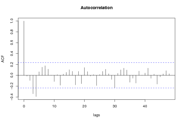
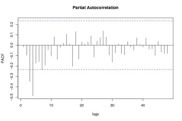
Title produced by software

(Partial) Autocorrelation Function

Date of computation

Sat, 13 Dec 2008 07:13:29 -0700

Cite this page as follows

Statistical Computations at FreeStatistics.org, Office for Research Development and Education, URL https://freestatistics.org/blog/index.php?v=date/2008/Dec/13/t12291776598lk4px22i6o8lbz.htm/, Retrieved Fri, 17 May 2024 02:39:14 +0000

Statistical Computations at FreeStatistics.org, Office for Research Development and Education, URL https://freestatistics.org/blog/index.php?pk=33111, Retrieved Fri, 17 May 2024 02:39:14 +0000

QR Codes:

Paste this QR Code to cite your computation.

Original text written by user:

IsPrivate?

No (this computation is public)

User-defined keywords

Estimated Impact

175

Family? (F = Feedback message, R = changed R code, M = changed R Module, P = changed Parameters, D = changed Data)

-     [(Partial) Autocorrelation Function] [ACF d=0 D=0 voor Xt] [2008-12-13 09:26:24] [b1bd16d1f47bfe13feacf1c27a0abba5]
-   PD  [(Partial) Autocorrelation Function] [ACF d=0 D=1] [2008-12-13 09:29:39] [b1bd16d1f47bfe13feacf1c27a0abba5]
-   PD    [(Partial) Autocorrelation Function] [step 1 ACF d=0 D=0] [2008-12-13 13:32:41] [b1bd16d1f47bfe13feacf1c27a0abba5]
-           [(Partial) Autocorrelation Function] [step 1 ACF d=1 D=0] [2008-12-13 13:35:54] [b1bd16d1f47bfe13feacf1c27a0abba5]
-             [(Partial) Autocorrelation Function] [step 1 ACF d=1 D=1] [2008-12-13 13:38:15] [b1bd16d1f47bfe13feacf1c27a0abba5]
-               [(Partial) Autocorrelation Function] [step 1 ACF d=1 D=2] [2008-12-13 13:42:02] [b1bd16d1f47bfe13feacf1c27a0abba5]
-                   [(Partial) Autocorrelation Function] [step 1 d=2 D=1] [2008-12-13 14:13:29] [e7b1048c2c3a353441b9143db4404b91] [Current]

Feedback Forum

Post a new message

Dataseries X:

Download CSV

Histogram

Boxplots

6.4
6.8
7.5
7.5
7.6
7.6
7.4
7.3
7.1
6.9
6.8
7.5
7.6
7.8
8
8.1
8.2
8.3
8.2
8
7.9
7.6
7.6
8.2
8.3
8.4
8.4
8.4
8.6
8.9
8.8
8.3
7.5
7.2
7.5
8.8
9.3
9.3
8.7
8.2
8.3
8.5
8.6
8.6
8.2
8.1
8
8.6
8.7
8.8
8.5
8.4
8.5
8.7
8.7
8.6
8.5
8.3
8.1
8.2
8.1
8.1
7.9
7.9
7.9
8
8
7.9
8
7.7
7.2
7.5
7.3
7
7
7
7.2
7.3
7.1
6.8
6.6
6.2
6.2
6.8

Summary of computational transaction
Raw Input	view raw input (R code)
Raw Output	view raw output of R engine
Computing time	1 seconds
R Server	'Sir Ronald Aylmer Fisher' @ 193.190.124.24

\begin{tabular}{lllllllll}
\hline
Summary of computational transaction \tabularnewline
Raw Input & view raw input (R code)  \tabularnewline
Raw Output & view raw output of R engine  \tabularnewline
Computing time & 1 seconds \tabularnewline
R Server & 'Sir Ronald Aylmer Fisher' @ 193.190.124.24 \tabularnewline
\hline
\end{tabular}
%Source: https://freestatistics.org/blog/index.php?pk=33111&T=0

[TABLE]
[ROW][C]Summary of computational transaction[/C][/ROW]
[ROW][C]Raw Input[/C][C]view raw input (R code) [/C][/ROW]
[ROW][C]Raw Output[/C][C]view raw output of R engine [/C][/ROW]
[ROW][C]Computing time[/C][C]1 seconds[/C][/ROW]
[ROW][C]R Server[/C][C]'Sir Ronald Aylmer Fisher' @ 193.190.124.24[/C][/ROW]
[/TABLE]
Source: https://freestatistics.org/blog/index.php?pk=33111&T=0

Globally Unique Identifier (entire table): ba.freestatistics.org/blog/index.php?pk=33111&T=0

As an alternative you can also use a QR Code:

The GUIDs for individual cells are displayed in the table below:

Summary of computational transaction
Raw Input	view raw input (R code)
Raw Output	view raw output of R engine
Computing time	1 seconds
R Server	'Sir Ronald Aylmer Fisher' @ 193.190.124.24

Autocorrelation Function
Time lag k	ACF(k)	T-STAT	P-value
1	-0.014863	-0.1244	0.450696
2	-0.095232	-0.7968	0.214139
3	-0.340584	-2.8495	0.002873
4	-0.391731	-3.2775	0.000816
5	0.065097	0.5446	0.293865
6	0.149832	1.2536	0.107082
7	0.177097	1.4817	0.071454
8	0.114018	0.9539	0.171698
9	0.003209	0.0269	0.489328
10	-0.114053	-0.9542	0.171625
11	0.011958	0.1001	0.460295
12	-0.182863	-1.5299	0.065269
13	0.022169	0.1855	0.426696
14	0.054426	0.4554	0.32513
15	0.103729	0.8679	0.194218
16	0.073403	0.6141	0.27056
17	-0.175723	-1.4702	0.072993
18	0.072898	0.6099	0.271948
19	-0.154311	-1.2911	0.100465
20	0.142892	1.1955	0.117959
21	0.068245	0.571	0.28492
22	-0.012854	-0.1075	0.457332
23	0.014167	0.1185	0.452992
24	-0.188934	-1.5807	0.059224
25	0.014515	0.1214	0.451844
26	0.072585	0.6073	0.272811
27	0.111783	0.9352	0.17644
28	0.028735	0.2404	0.405356
29	-0.076595	-0.6408	0.261861
30	-0.22807	-1.9082	0.030235
31	0.037719	0.3156	0.37663
32	0.101755	0.8513	0.198741
33	0.131821	1.1029	0.136926
34	0.097598	0.8166	0.208474
35	-0.12815	-1.0722	0.14366
36	-0.053887	-0.4508	0.326746
37	-0.144362	-1.2078	0.115591
38	0.078325	0.6553	0.257206
39	0.002583	0.0216	0.49141
40	0.041659	0.3485	0.36424
41	0.132238	1.1064	0.136174
42	-0.054913	-0.4594	0.323673
43	0.022273	0.1863	0.426355
44	-0.161834	-1.354	0.090046
45	-0.028761	-0.2406	0.405272
46	0.026387	0.2208	0.412958
47	0.085796	0.7178	0.237628
48	0.029292	0.2451	0.403559

\begin{tabular}{lllllllll}
\hline
Autocorrelation Function \tabularnewline
Time lag k & ACF(k) & T-STAT & P-value \tabularnewline
1 & -0.014863 & -0.1244 & 0.450696 \tabularnewline
2 & -0.095232 & -0.7968 & 0.214139 \tabularnewline
3 & -0.340584 & -2.8495 & 0.002873 \tabularnewline
4 & -0.391731 & -3.2775 & 0.000816 \tabularnewline
5 & 0.065097 & 0.5446 & 0.293865 \tabularnewline
6 & 0.149832 & 1.2536 & 0.107082 \tabularnewline
7 & 0.177097 & 1.4817 & 0.071454 \tabularnewline
8 & 0.114018 & 0.9539 & 0.171698 \tabularnewline
9 & 0.003209 & 0.0269 & 0.489328 \tabularnewline
10 & -0.114053 & -0.9542 & 0.171625 \tabularnewline
11 & 0.011958 & 0.1001 & 0.460295 \tabularnewline
12 & -0.182863 & -1.5299 & 0.065269 \tabularnewline
13 & 0.022169 & 0.1855 & 0.426696 \tabularnewline
14 & 0.054426 & 0.4554 & 0.32513 \tabularnewline
15 & 0.103729 & 0.8679 & 0.194218 \tabularnewline
16 & 0.073403 & 0.6141 & 0.27056 \tabularnewline
17 & -0.175723 & -1.4702 & 0.072993 \tabularnewline
18 & 0.072898 & 0.6099 & 0.271948 \tabularnewline
19 & -0.154311 & -1.2911 & 0.100465 \tabularnewline
20 & 0.142892 & 1.1955 & 0.117959 \tabularnewline
21 & 0.068245 & 0.571 & 0.28492 \tabularnewline
22 & -0.012854 & -0.1075 & 0.457332 \tabularnewline
23 & 0.014167 & 0.1185 & 0.452992 \tabularnewline
24 & -0.188934 & -1.5807 & 0.059224 \tabularnewline
25 & 0.014515 & 0.1214 & 0.451844 \tabularnewline
26 & 0.072585 & 0.6073 & 0.272811 \tabularnewline
27 & 0.111783 & 0.9352 & 0.17644 \tabularnewline
28 & 0.028735 & 0.2404 & 0.405356 \tabularnewline
29 & -0.076595 & -0.6408 & 0.261861 \tabularnewline
30 & -0.22807 & -1.9082 & 0.030235 \tabularnewline
31 & 0.037719 & 0.3156 & 0.37663 \tabularnewline
32 & 0.101755 & 0.8513 & 0.198741 \tabularnewline
33 & 0.131821 & 1.1029 & 0.136926 \tabularnewline
34 & 0.097598 & 0.8166 & 0.208474 \tabularnewline
35 & -0.12815 & -1.0722 & 0.14366 \tabularnewline
36 & -0.053887 & -0.4508 & 0.326746 \tabularnewline
37 & -0.144362 & -1.2078 & 0.115591 \tabularnewline
38 & 0.078325 & 0.6553 & 0.257206 \tabularnewline
39 & 0.002583 & 0.0216 & 0.49141 \tabularnewline
40 & 0.041659 & 0.3485 & 0.36424 \tabularnewline
41 & 0.132238 & 1.1064 & 0.136174 \tabularnewline
42 & -0.054913 & -0.4594 & 0.323673 \tabularnewline
43 & 0.022273 & 0.1863 & 0.426355 \tabularnewline
44 & -0.161834 & -1.354 & 0.090046 \tabularnewline
45 & -0.028761 & -0.2406 & 0.405272 \tabularnewline
46 & 0.026387 & 0.2208 & 0.412958 \tabularnewline
47 & 0.085796 & 0.7178 & 0.237628 \tabularnewline
48 & 0.029292 & 0.2451 & 0.403559 \tabularnewline
\hline
\end{tabular}
%Source: https://freestatistics.org/blog/index.php?pk=33111&T=1

[TABLE]
[ROW][C]Autocorrelation Function[/C][/ROW]
[ROW][C]Time lag k[/C][C]ACF(k)[/C][C]T-STAT[/C][C]P-value[/C][/ROW]
[ROW][C]1[/C][C]-0.014863[/C][C]-0.1244[/C][C]0.450696[/C][/ROW]
[ROW][C]2[/C][C]-0.095232[/C][C]-0.7968[/C][C]0.214139[/C][/ROW]
[ROW][C]3[/C][C]-0.340584[/C][C]-2.8495[/C][C]0.002873[/C][/ROW]
[ROW][C]4[/C][C]-0.391731[/C][C]-3.2775[/C][C]0.000816[/C][/ROW]
[ROW][C]5[/C][C]0.065097[/C][C]0.5446[/C][C]0.293865[/C][/ROW]
[ROW][C]6[/C][C]0.149832[/C][C]1.2536[/C][C]0.107082[/C][/ROW]
[ROW][C]7[/C][C]0.177097[/C][C]1.4817[/C][C]0.071454[/C][/ROW]
[ROW][C]8[/C][C]0.114018[/C][C]0.9539[/C][C]0.171698[/C][/ROW]
[ROW][C]9[/C][C]0.003209[/C][C]0.0269[/C][C]0.489328[/C][/ROW]
[ROW][C]10[/C][C]-0.114053[/C][C]-0.9542[/C][C]0.171625[/C][/ROW]
[ROW][C]11[/C][C]0.011958[/C][C]0.1001[/C][C]0.460295[/C][/ROW]
[ROW][C]12[/C][C]-0.182863[/C][C]-1.5299[/C][C]0.065269[/C][/ROW]
[ROW][C]13[/C][C]0.022169[/C][C]0.1855[/C][C]0.426696[/C][/ROW]
[ROW][C]14[/C][C]0.054426[/C][C]0.4554[/C][C]0.32513[/C][/ROW]
[ROW][C]15[/C][C]0.103729[/C][C]0.8679[/C][C]0.194218[/C][/ROW]
[ROW][C]16[/C][C]0.073403[/C][C]0.6141[/C][C]0.27056[/C][/ROW]
[ROW][C]17[/C][C]-0.175723[/C][C]-1.4702[/C][C]0.072993[/C][/ROW]
[ROW][C]18[/C][C]0.072898[/C][C]0.6099[/C][C]0.271948[/C][/ROW]
[ROW][C]19[/C][C]-0.154311[/C][C]-1.2911[/C][C]0.100465[/C][/ROW]
[ROW][C]20[/C][C]0.142892[/C][C]1.1955[/C][C]0.117959[/C][/ROW]
[ROW][C]21[/C][C]0.068245[/C][C]0.571[/C][C]0.28492[/C][/ROW]
[ROW][C]22[/C][C]-0.012854[/C][C]-0.1075[/C][C]0.457332[/C][/ROW]
[ROW][C]23[/C][C]0.014167[/C][C]0.1185[/C][C]0.452992[/C][/ROW]
[ROW][C]24[/C][C]-0.188934[/C][C]-1.5807[/C][C]0.059224[/C][/ROW]
[ROW][C]25[/C][C]0.014515[/C][C]0.1214[/C][C]0.451844[/C][/ROW]
[ROW][C]26[/C][C]0.072585[/C][C]0.6073[/C][C]0.272811[/C][/ROW]
[ROW][C]27[/C][C]0.111783[/C][C]0.9352[/C][C]0.17644[/C][/ROW]
[ROW][C]28[/C][C]0.028735[/C][C]0.2404[/C][C]0.405356[/C][/ROW]
[ROW][C]29[/C][C]-0.076595[/C][C]-0.6408[/C][C]0.261861[/C][/ROW]
[ROW][C]30[/C][C]-0.22807[/C][C]-1.9082[/C][C]0.030235[/C][/ROW]
[ROW][C]31[/C][C]0.037719[/C][C]0.3156[/C][C]0.37663[/C][/ROW]
[ROW][C]32[/C][C]0.101755[/C][C]0.8513[/C][C]0.198741[/C][/ROW]
[ROW][C]33[/C][C]0.131821[/C][C]1.1029[/C][C]0.136926[/C][/ROW]
[ROW][C]34[/C][C]0.097598[/C][C]0.8166[/C][C]0.208474[/C][/ROW]
[ROW][C]35[/C][C]-0.12815[/C][C]-1.0722[/C][C]0.14366[/C][/ROW]
[ROW][C]36[/C][C]-0.053887[/C][C]-0.4508[/C][C]0.326746[/C][/ROW]
[ROW][C]37[/C][C]-0.144362[/C][C]-1.2078[/C][C]0.115591[/C][/ROW]
[ROW][C]38[/C][C]0.078325[/C][C]0.6553[/C][C]0.257206[/C][/ROW]
[ROW][C]39[/C][C]0.002583[/C][C]0.0216[/C][C]0.49141[/C][/ROW]
[ROW][C]40[/C][C]0.041659[/C][C]0.3485[/C][C]0.36424[/C][/ROW]
[ROW][C]41[/C][C]0.132238[/C][C]1.1064[/C][C]0.136174[/C][/ROW]
[ROW][C]42[/C][C]-0.054913[/C][C]-0.4594[/C][C]0.323673[/C][/ROW]
[ROW][C]43[/C][C]0.022273[/C][C]0.1863[/C][C]0.426355[/C][/ROW]
[ROW][C]44[/C][C]-0.161834[/C][C]-1.354[/C][C]0.090046[/C][/ROW]
[ROW][C]45[/C][C]-0.028761[/C][C]-0.2406[/C][C]0.405272[/C][/ROW]
[ROW][C]46[/C][C]0.026387[/C][C]0.2208[/C][C]0.412958[/C][/ROW]
[ROW][C]47[/C][C]0.085796[/C][C]0.7178[/C][C]0.237628[/C][/ROW]
[ROW][C]48[/C][C]0.029292[/C][C]0.2451[/C][C]0.403559[/C][/ROW]
[/TABLE]
Source: https://freestatistics.org/blog/index.php?pk=33111&T=1

Globally Unique Identifier (entire table): ba.freestatistics.org/blog/index.php?pk=33111&T=1

As an alternative you can also use a QR Code:

The GUIDs for individual cells are displayed in the table below:

Autocorrelation Function
Time lag k	ACF(k)	T-STAT	P-value
1	-0.014863	-0.1244	0.450696
2	-0.095232	-0.7968	0.214139
3	-0.340584	-2.8495	0.002873
4	-0.391731	-3.2775	0.000816
5	0.065097	0.5446	0.293865
6	0.149832	1.2536	0.107082
7	0.177097	1.4817	0.071454
8	0.114018	0.9539	0.171698
9	0.003209	0.0269	0.489328
10	-0.114053	-0.9542	0.171625
11	0.011958	0.1001	0.460295
12	-0.182863	-1.5299	0.065269
13	0.022169	0.1855	0.426696
14	0.054426	0.4554	0.32513
15	0.103729	0.8679	0.194218
16	0.073403	0.6141	0.27056
17	-0.175723	-1.4702	0.072993
18	0.072898	0.6099	0.271948
19	-0.154311	-1.2911	0.100465
20	0.142892	1.1955	0.117959
21	0.068245	0.571	0.28492
22	-0.012854	-0.1075	0.457332
23	0.014167	0.1185	0.452992
24	-0.188934	-1.5807	0.059224
25	0.014515	0.1214	0.451844
26	0.072585	0.6073	0.272811
27	0.111783	0.9352	0.17644
28	0.028735	0.2404	0.405356
29	-0.076595	-0.6408	0.261861
30	-0.22807	-1.9082	0.030235
31	0.037719	0.3156	0.37663
32	0.101755	0.8513	0.198741
33	0.131821	1.1029	0.136926
34	0.097598	0.8166	0.208474
35	-0.12815	-1.0722	0.14366
36	-0.053887	-0.4508	0.326746
37	-0.144362	-1.2078	0.115591
38	0.078325	0.6553	0.257206
39	0.002583	0.0216	0.49141
40	0.041659	0.3485	0.36424
41	0.132238	1.1064	0.136174
42	-0.054913	-0.4594	0.323673
43	0.022273	0.1863	0.426355
44	-0.161834	-1.354	0.090046
45	-0.028761	-0.2406	0.405272
46	0.026387	0.2208	0.412958
47	0.085796	0.7178	0.237628
48	0.029292	0.2451	0.403559

Partial Autocorrelation Function
Time lag k	PACF(k)	T-STAT	P-value
1	-0.014863	-0.1244	0.450696
2	-0.095474	-0.7988	0.213556
3	-0.34679	-2.9015	0.002481
4	-0.485743	-4.064	6.2e-05
5	-0.171106	-1.4316	0.078358
6	-0.15729	-1.316	0.096237
7	-0.233148	-1.9507	0.027551
8	-0.192422	-1.6099	0.055958
9	-0.041411	-0.3465	0.365015
10	-0.102297	-0.8559	0.197494
11	0.078785	0.6592	0.255977
12	-0.133422	-1.1163	0.134057
13	-0.019536	-0.1635	0.435316
14	0.020389	0.1706	0.432522
15	0.106895	0.8943	0.187101
16	0.01216	0.1017	0.459629
17	-0.202323	-1.6928	0.047474
18	0.131779	1.1025	0.137002
19	-0.131077	-1.0967	0.138272
20	0.031647	0.2648	0.395979
21	0.015596	0.1305	0.448278
22	0.032822	0.2746	0.392214
23	0.089045	0.745	0.229381
24	-0.113138	-0.9466	0.173554
25	0.040776	0.3412	0.367004
26	0.074586	0.624	0.267317
27	0.135838	1.1365	0.129811
28	0.078112	0.6535	0.257777
29	-0.095792	-0.8015	0.212791
30	-0.161772	-1.3535	0.090128
31	-0.072353	-0.6053	0.273452
32	0.012014	0.1005	0.460112
33	-0.078672	-0.6582	0.256279
34	-0.090414	-0.7565	0.225957
35	0.034596	0.2894	0.386547
36	-0.017862	-0.1494	0.440817
37	-0.047849	-0.4003	0.345064
38	0.070792	0.5923	0.277783
39	0.007778	0.0651	0.47415
40	-0.017427	-0.1458	0.442247
41	0.070619	0.5908	0.278264
42	-0.036893	-0.3087	0.379246
43	-0.035235	-0.2948	0.38451
44	-0.096455	-0.807	0.211199
45	0.036646	0.3066	0.380028
46	-0.065275	-0.5461	0.293355
47	-0.077756	-0.6505	0.258733
48	-0.07906	-0.6615	0.255244

\begin{tabular}{lllllllll}
\hline
Partial Autocorrelation Function \tabularnewline
Time lag k & PACF(k) & T-STAT & P-value \tabularnewline
1 & -0.014863 & -0.1244 & 0.450696 \tabularnewline
2 & -0.095474 & -0.7988 & 0.213556 \tabularnewline
3 & -0.34679 & -2.9015 & 0.002481 \tabularnewline
4 & -0.485743 & -4.064 & 6.2e-05 \tabularnewline
5 & -0.171106 & -1.4316 & 0.078358 \tabularnewline
6 & -0.15729 & -1.316 & 0.096237 \tabularnewline
7 & -0.233148 & -1.9507 & 0.027551 \tabularnewline
8 & -0.192422 & -1.6099 & 0.055958 \tabularnewline
9 & -0.041411 & -0.3465 & 0.365015 \tabularnewline
10 & -0.102297 & -0.8559 & 0.197494 \tabularnewline
11 & 0.078785 & 0.6592 & 0.255977 \tabularnewline
12 & -0.133422 & -1.1163 & 0.134057 \tabularnewline
13 & -0.019536 & -0.1635 & 0.435316 \tabularnewline
14 & 0.020389 & 0.1706 & 0.432522 \tabularnewline
15 & 0.106895 & 0.8943 & 0.187101 \tabularnewline
16 & 0.01216 & 0.1017 & 0.459629 \tabularnewline
17 & -0.202323 & -1.6928 & 0.047474 \tabularnewline
18 & 0.131779 & 1.1025 & 0.137002 \tabularnewline
19 & -0.131077 & -1.0967 & 0.138272 \tabularnewline
20 & 0.031647 & 0.2648 & 0.395979 \tabularnewline
21 & 0.015596 & 0.1305 & 0.448278 \tabularnewline
22 & 0.032822 & 0.2746 & 0.392214 \tabularnewline
23 & 0.089045 & 0.745 & 0.229381 \tabularnewline
24 & -0.113138 & -0.9466 & 0.173554 \tabularnewline
25 & 0.040776 & 0.3412 & 0.367004 \tabularnewline
26 & 0.074586 & 0.624 & 0.267317 \tabularnewline
27 & 0.135838 & 1.1365 & 0.129811 \tabularnewline
28 & 0.078112 & 0.6535 & 0.257777 \tabularnewline
29 & -0.095792 & -0.8015 & 0.212791 \tabularnewline
30 & -0.161772 & -1.3535 & 0.090128 \tabularnewline
31 & -0.072353 & -0.6053 & 0.273452 \tabularnewline
32 & 0.012014 & 0.1005 & 0.460112 \tabularnewline
33 & -0.078672 & -0.6582 & 0.256279 \tabularnewline
34 & -0.090414 & -0.7565 & 0.225957 \tabularnewline
35 & 0.034596 & 0.2894 & 0.386547 \tabularnewline
36 & -0.017862 & -0.1494 & 0.440817 \tabularnewline
37 & -0.047849 & -0.4003 & 0.345064 \tabularnewline
38 & 0.070792 & 0.5923 & 0.277783 \tabularnewline
39 & 0.007778 & 0.0651 & 0.47415 \tabularnewline
40 & -0.017427 & -0.1458 & 0.442247 \tabularnewline
41 & 0.070619 & 0.5908 & 0.278264 \tabularnewline
42 & -0.036893 & -0.3087 & 0.379246 \tabularnewline
43 & -0.035235 & -0.2948 & 0.38451 \tabularnewline
44 & -0.096455 & -0.807 & 0.211199 \tabularnewline
45 & 0.036646 & 0.3066 & 0.380028 \tabularnewline
46 & -0.065275 & -0.5461 & 0.293355 \tabularnewline
47 & -0.077756 & -0.6505 & 0.258733 \tabularnewline
48 & -0.07906 & -0.6615 & 0.255244 \tabularnewline
\hline
\end{tabular}
%Source: https://freestatistics.org/blog/index.php?pk=33111&T=2

[TABLE]
[ROW][C]Partial Autocorrelation Function[/C][/ROW]
[ROW][C]Time lag k[/C][C]PACF(k)[/C][C]T-STAT[/C][C]P-value[/C][/ROW]
[ROW][C]1[/C][C]-0.014863[/C][C]-0.1244[/C][C]0.450696[/C][/ROW]
[ROW][C]2[/C][C]-0.095474[/C][C]-0.7988[/C][C]0.213556[/C][/ROW]
[ROW][C]3[/C][C]-0.34679[/C][C]-2.9015[/C][C]0.002481[/C][/ROW]
[ROW][C]4[/C][C]-0.485743[/C][C]-4.064[/C][C]6.2e-05[/C][/ROW]
[ROW][C]5[/C][C]-0.171106[/C][C]-1.4316[/C][C]0.078358[/C][/ROW]
[ROW][C]6[/C][C]-0.15729[/C][C]-1.316[/C][C]0.096237[/C][/ROW]
[ROW][C]7[/C][C]-0.233148[/C][C]-1.9507[/C][C]0.027551[/C][/ROW]
[ROW][C]8[/C][C]-0.192422[/C][C]-1.6099[/C][C]0.055958[/C][/ROW]
[ROW][C]9[/C][C]-0.041411[/C][C]-0.3465[/C][C]0.365015[/C][/ROW]
[ROW][C]10[/C][C]-0.102297[/C][C]-0.8559[/C][C]0.197494[/C][/ROW]
[ROW][C]11[/C][C]0.078785[/C][C]0.6592[/C][C]0.255977[/C][/ROW]
[ROW][C]12[/C][C]-0.133422[/C][C]-1.1163[/C][C]0.134057[/C][/ROW]
[ROW][C]13[/C][C]-0.019536[/C][C]-0.1635[/C][C]0.435316[/C][/ROW]
[ROW][C]14[/C][C]0.020389[/C][C]0.1706[/C][C]0.432522[/C][/ROW]
[ROW][C]15[/C][C]0.106895[/C][C]0.8943[/C][C]0.187101[/C][/ROW]
[ROW][C]16[/C][C]0.01216[/C][C]0.1017[/C][C]0.459629[/C][/ROW]
[ROW][C]17[/C][C]-0.202323[/C][C]-1.6928[/C][C]0.047474[/C][/ROW]
[ROW][C]18[/C][C]0.131779[/C][C]1.1025[/C][C]0.137002[/C][/ROW]
[ROW][C]19[/C][C]-0.131077[/C][C]-1.0967[/C][C]0.138272[/C][/ROW]
[ROW][C]20[/C][C]0.031647[/C][C]0.2648[/C][C]0.395979[/C][/ROW]
[ROW][C]21[/C][C]0.015596[/C][C]0.1305[/C][C]0.448278[/C][/ROW]
[ROW][C]22[/C][C]0.032822[/C][C]0.2746[/C][C]0.392214[/C][/ROW]
[ROW][C]23[/C][C]0.089045[/C][C]0.745[/C][C]0.229381[/C][/ROW]
[ROW][C]24[/C][C]-0.113138[/C][C]-0.9466[/C][C]0.173554[/C][/ROW]
[ROW][C]25[/C][C]0.040776[/C][C]0.3412[/C][C]0.367004[/C][/ROW]
[ROW][C]26[/C][C]0.074586[/C][C]0.624[/C][C]0.267317[/C][/ROW]
[ROW][C]27[/C][C]0.135838[/C][C]1.1365[/C][C]0.129811[/C][/ROW]
[ROW][C]28[/C][C]0.078112[/C][C]0.6535[/C][C]0.257777[/C][/ROW]
[ROW][C]29[/C][C]-0.095792[/C][C]-0.8015[/C][C]0.212791[/C][/ROW]
[ROW][C]30[/C][C]-0.161772[/C][C]-1.3535[/C][C]0.090128[/C][/ROW]
[ROW][C]31[/C][C]-0.072353[/C][C]-0.6053[/C][C]0.273452[/C][/ROW]
[ROW][C]32[/C][C]0.012014[/C][C]0.1005[/C][C]0.460112[/C][/ROW]
[ROW][C]33[/C][C]-0.078672[/C][C]-0.6582[/C][C]0.256279[/C][/ROW]
[ROW][C]34[/C][C]-0.090414[/C][C]-0.7565[/C][C]0.225957[/C][/ROW]
[ROW][C]35[/C][C]0.034596[/C][C]0.2894[/C][C]0.386547[/C][/ROW]
[ROW][C]36[/C][C]-0.017862[/C][C]-0.1494[/C][C]0.440817[/C][/ROW]
[ROW][C]37[/C][C]-0.047849[/C][C]-0.4003[/C][C]0.345064[/C][/ROW]
[ROW][C]38[/C][C]0.070792[/C][C]0.5923[/C][C]0.277783[/C][/ROW]
[ROW][C]39[/C][C]0.007778[/C][C]0.0651[/C][C]0.47415[/C][/ROW]
[ROW][C]40[/C][C]-0.017427[/C][C]-0.1458[/C][C]0.442247[/C][/ROW]
[ROW][C]41[/C][C]0.070619[/C][C]0.5908[/C][C]0.278264[/C][/ROW]
[ROW][C]42[/C][C]-0.036893[/C][C]-0.3087[/C][C]0.379246[/C][/ROW]
[ROW][C]43[/C][C]-0.035235[/C][C]-0.2948[/C][C]0.38451[/C][/ROW]
[ROW][C]44[/C][C]-0.096455[/C][C]-0.807[/C][C]0.211199[/C][/ROW]
[ROW][C]45[/C][C]0.036646[/C][C]0.3066[/C][C]0.380028[/C][/ROW]
[ROW][C]46[/C][C]-0.065275[/C][C]-0.5461[/C][C]0.293355[/C][/ROW]
[ROW][C]47[/C][C]-0.077756[/C][C]-0.6505[/C][C]0.258733[/C][/ROW]
[ROW][C]48[/C][C]-0.07906[/C][C]-0.6615[/C][C]0.255244[/C][/ROW]
[/TABLE]
Source: https://freestatistics.org/blog/index.php?pk=33111&T=2

Globally Unique Identifier (entire table): ba.freestatistics.org/blog/index.php?pk=33111&T=2

As an alternative you can also use a QR Code:

The GUIDs for individual cells are displayed in the table below:

Partial Autocorrelation Function
Time lag k	PACF(k)	T-STAT	P-value
1	-0.014863	-0.1244	0.450696
2	-0.095474	-0.7988	0.213556
3	-0.34679	-2.9015	0.002481
4	-0.485743	-4.064	6.2e-05
5	-0.171106	-1.4316	0.078358
6	-0.15729	-1.316	0.096237
7	-0.233148	-1.9507	0.027551
8	-0.192422	-1.6099	0.055958
9	-0.041411	-0.3465	0.365015
10	-0.102297	-0.8559	0.197494
11	0.078785	0.6592	0.255977
12	-0.133422	-1.1163	0.134057
13	-0.019536	-0.1635	0.435316
14	0.020389	0.1706	0.432522
15	0.106895	0.8943	0.187101
16	0.01216	0.1017	0.459629
17	-0.202323	-1.6928	0.047474
18	0.131779	1.1025	0.137002
19	-0.131077	-1.0967	0.138272
20	0.031647	0.2648	0.395979
21	0.015596	0.1305	0.448278
22	0.032822	0.2746	0.392214
23	0.089045	0.745	0.229381
24	-0.113138	-0.9466	0.173554
25	0.040776	0.3412	0.367004
26	0.074586	0.624	0.267317
27	0.135838	1.1365	0.129811
28	0.078112	0.6535	0.257777
29	-0.095792	-0.8015	0.212791
30	-0.161772	-1.3535	0.090128
31	-0.072353	-0.6053	0.273452
32	0.012014	0.1005	0.460112
33	-0.078672	-0.6582	0.256279
34	-0.090414	-0.7565	0.225957
35	0.034596	0.2894	0.386547
36	-0.017862	-0.1494	0.440817
37	-0.047849	-0.4003	0.345064
38	0.070792	0.5923	0.277783
39	0.007778	0.0651	0.47415
40	-0.017427	-0.1458	0.442247
41	0.070619	0.5908	0.278264
42	-0.036893	-0.3087	0.379246
43	-0.035235	-0.2948	0.38451
44	-0.096455	-0.807	0.211199
45	0.036646	0.3066	0.380028
46	-0.065275	-0.5461	0.293355
47	-0.077756	-0.6505	0.258733
48	-0.07906	-0.6615	0.255244

Figure 1

PNG link

Postscript link

PDF link

Figure 2

PNG link

Postscript link

PDF link

Parameters (Session):

par1 = 1 ; par2 = 0 ; par3 = 2 ; par4 = 12 ;

Parameters (R input):

par1 = 48 ; par2 = 1 ; par3 = 2 ; par4 = 1 ; par5 = 12 ;

R code (references can be found in the software module):

if (par1 == 'Default') {
par1 = 10*log10(length(x))
} else {
par1 <- as.numeric(par1)
}
par2 <- as.numeric(par2)
par3 <- as.numeric(par3)
par4 <- as.numeric(par4)
par5 <- as.numeric(par5)
if (par2 == 0) {
x <- log(x)
} else {
x <- (x ^ par2 - 1) / par2
}
if (par3 > 0) x <- diff(x,lag=1,difference=par3)
if (par4 > 0) x <- diff(x,lag=par5,difference=par4)
bitmap(file='pic1.png')
racf <- acf(x,par1,main='Autocorrelation',xlab='lags',ylab='ACF')
dev.off()
bitmap(file='pic2.png')
rpacf <- pacf(x,par1,main='Partial Autocorrelation',xlab='lags',ylab='PACF')
dev.off()
(myacf <- c(racf$acf))
(mypacf <- c(rpacf$acf))
lengthx <- length(x)
sqrtn <- sqrt(lengthx)
load(file='createtable')
a<-table.start()
a<-table.row.start(a)
a<-table.element(a,'Autocorrelation Function',4,TRUE)
a<-table.row.end(a)
a<-table.row.start(a)
a<-table.element(a,'Time lag k',header=TRUE)
a<-table.element(a,hyperlink('basics.htm','ACF(k)','click here for more information about the Autocorrelation Function'),header=TRUE)
a<-table.element(a,'T-STAT',header=TRUE)
a<-table.element(a,'P-value',header=TRUE)
a<-table.row.end(a)
for (i in 2:(par1+1)) {
a<-table.row.start(a)
a<-table.element(a,i-1,header=TRUE)
a<-table.element(a,round(myacf[i],6))
mytstat <- myacf[i]*sqrtn
a<-table.element(a,round(mytstat,4))
a<-table.element(a,round(1-pt(abs(mytstat),lengthx),6))
a<-table.row.end(a)
}
a<-table.end(a)
table.save(a,file='mytable.tab')
a<-table.start()
a<-table.row.start(a)
a<-table.element(a,'Partial Autocorrelation Function',4,TRUE)
a<-table.row.end(a)
a<-table.row.start(a)
a<-table.element(a,'Time lag k',header=TRUE)
a<-table.element(a,hyperlink('basics.htm','PACF(k)','click here for more information about the Partial Autocorrelation Function'),header=TRUE)
a<-table.element(a,'T-STAT',header=TRUE)
a<-table.element(a,'P-value',header=TRUE)
a<-table.row.end(a)
for (i in 1:par1) {
a<-table.row.start(a)
a<-table.element(a,i,header=TRUE)
a<-table.element(a,round(mypacf[i],6))
mytstat <- mypacf[i]*sqrtn
a<-table.element(a,round(mytstat,4))
a<-table.element(a,round(1-pt(abs(mytstat),lengthx),6))
a<-table.row.end(a)
}
a<-table.end(a)
table.save(a,file='mytable1.tab')

Free Statistics

Description of Statistical Computation

Tree of Dependent Computations

Dataset

Tables (Output of Computation)

Figures (Output of Computation)

Input Parameters & R Code