Repository of Reproducible Computations

Free Statistics

of Irreproducible Research!

Author's title

Author

*The author of this computation has been verified*

R Software Module

rwasp_autocorrelation.wasp

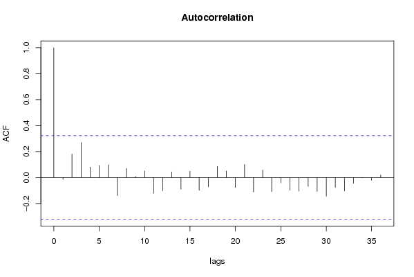
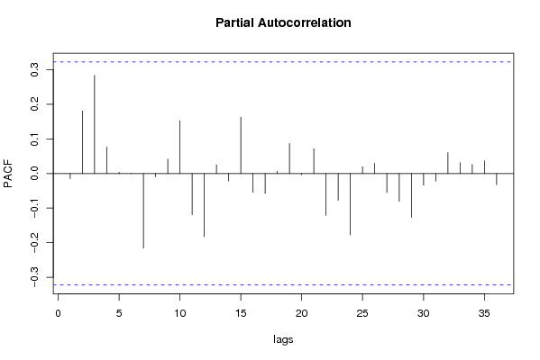
Title produced by software

(Partial) Autocorrelation Function

Date of computation

Wed, 10 Dec 2008 13:40:13 -0700

Cite this page as follows

Statistical Computations at FreeStatistics.org, Office for Research Development and Education, URL https://freestatistics.org/blog/index.php?v=date/2008/Dec/10/t1228941660pp20e33ylrcma50.htm/, Retrieved Fri, 17 May 2024 01:41:08 +0000

Statistical Computations at FreeStatistics.org, Office for Research Development and Education, URL https://freestatistics.org/blog/index.php?pk=32106, Retrieved Fri, 17 May 2024 01:41:08 +0000

QR Codes:

Paste this QR Code to cite your computation.

Original text written by user:

IsPrivate?

No (this computation is public)

User-defined keywords

Estimated Impact

176

Family? (F = Feedback message, R = changed R code, M = changed R Module, P = changed Parameters, D = changed Data)

-     [Maximum-likelihood Fitting - Normal Distribution] [Maximum-likelihoo...] [2008-12-10 19:35:16] [82d201ca7b4e7cd2c6f885d29b5b6937]
- RMP   [(Partial) Autocorrelation Function] [P(ACF)] [2008-12-10 20:35:05] [82d201ca7b4e7cd2c6f885d29b5b6937]
-           [(Partial) Autocorrelation Function] [(P)ACF] [2008-12-10 20:40:13] [00a0a665d7a07edd2e460056b0c0c354] [Current]
- RM          [Spectral Analysis] [Spectrum] [2008-12-10 20:49:46] [82d201ca7b4e7cd2c6f885d29b5b6937] 
-               [Spectral Analysis] [P(ACF)] [2008-12-10 20:54:47] [82d201ca7b4e7cd2c6f885d29b5b6937] 
-   P             [Spectral Analysis] [spectrum] [2008-12-13 16:09:22] [82d201ca7b4e7cd2c6f885d29b5b6937] 
-   P               [Spectral Analysis] [spectrum] [2008-12-13 16:11:43] [82d201ca7b4e7cd2c6f885d29b5b6937] 
-   PD                [Spectral Analysis] [spectrum : invoer] [2008-12-14 13:25:58] [82d201ca7b4e7cd2c6f885d29b5b6937] 

Feedback Forum

Post a new message

Dataseries X:

Download CSV

Histogram

Boxplots

Summary of computational transaction
Raw Input	view raw input (R code)
Raw Output	view raw output of R engine
Computing time	2 seconds
R Server	'Sir Ronald Aylmer Fisher' @ 193.190.124.24

\begin{tabular}{lllllllll}
\hline
Summary of computational transaction \tabularnewline
Raw Input & view raw input (R code)  \tabularnewline
Raw Output & view raw output of R engine  \tabularnewline
Computing time & 2 seconds \tabularnewline
R Server & 'Sir Ronald Aylmer Fisher' @ 193.190.124.24 \tabularnewline
\hline
\end{tabular}
%Source: https://freestatistics.org/blog/index.php?pk=32106&T=0

[TABLE]
[ROW][C]Summary of computational transaction[/C][/ROW]
[ROW][C]Raw Input[/C][C]view raw input (R code) [/C][/ROW]
[ROW][C]Raw Output[/C][C]view raw output of R engine [/C][/ROW]
[ROW][C]Computing time[/C][C]2 seconds[/C][/ROW]
[ROW][C]R Server[/C][C]'Sir Ronald Aylmer Fisher' @ 193.190.124.24[/C][/ROW]
[/TABLE]
Source: https://freestatistics.org/blog/index.php?pk=32106&T=0

Globally Unique Identifier (entire table): ba.freestatistics.org/blog/index.php?pk=32106&T=0

As an alternative you can also use a QR Code:

The GUIDs for individual cells are displayed in the table below:

Summary of computational transaction
Raw Input	view raw input (R code)
Raw Output	view raw output of R engine
Computing time	2 seconds
R Server	'Sir Ronald Aylmer Fisher' @ 193.190.124.24

Autocorrelation Function
Time lag k	ACF(k)	T-STAT	P-value
1	-0.014738	-0.0896	0.464525
2	0.180958	1.1007	0.139063
3	0.269388	1.6386	0.054885
4	0.079869	0.4858	0.314979
5	0.092871	0.5649	0.287771
6	0.09759	0.5936	0.27819
7	-0.139327	-0.8475	0.201084
8	0.070229	0.4272	0.335861
9	0.008385	0.051	0.479799
10	0.050234	0.3056	0.380825
11	-0.121289	-0.7378	0.232654
12	-0.102028	-0.6206	0.26933
13	0.043231	0.263	0.397018
14	-0.089994	-0.5474	0.293692
15	0.048842	0.2971	0.384028
16	-0.099206	-0.6034	0.274946
17	-0.071538	-0.4351	0.332991
18	0.084367	0.5132	0.305436
19	0.049634	0.3019	0.382206
20	-0.076629	-0.4661	0.321932
21	0.100829	0.6133	0.271709
22	-0.111916	-0.6808	0.250131
23	0.056965	0.3465	0.365463
24	-0.109019	-0.6631	0.255678
25	-0.041782	-0.2542	0.400392
26	-0.09915	-0.6031	0.275059
27	-0.105143	-0.6396	0.263199
28	-0.067712	-0.4119	0.341403
29	-0.108272	-0.6586	0.257118
30	-0.144556	-0.8793	0.192457
31	-0.075725	-0.4606	0.323884
32	-0.104072	-0.633	0.2653
33	-0.045234	-0.2751	0.392366
34	-0.003124	-0.019	0.492471
35	-0.022057	-0.1342	0.447
36	0.019119	0.1163	0.454024
37	NA	NA	NA
38	NA	NA	NA
39	NA	NA	NA
40	NA	NA	NA
41	NA	NA	NA
42	NA	NA	NA
43	NA	NA	NA
44	NA	NA	NA
45	NA	NA	NA
46	NA	NA	NA
47	NA	NA	NA
48	NA	NA	NA

\begin{tabular}{lllllllll}
\hline
Autocorrelation Function \tabularnewline
Time lag k & ACF(k) & T-STAT & P-value \tabularnewline
1 & -0.014738 & -0.0896 & 0.464525 \tabularnewline
2 & 0.180958 & 1.1007 & 0.139063 \tabularnewline
3 & 0.269388 & 1.6386 & 0.054885 \tabularnewline
4 & 0.079869 & 0.4858 & 0.314979 \tabularnewline
5 & 0.092871 & 0.5649 & 0.287771 \tabularnewline
6 & 0.09759 & 0.5936 & 0.27819 \tabularnewline
7 & -0.139327 & -0.8475 & 0.201084 \tabularnewline
8 & 0.070229 & 0.4272 & 0.335861 \tabularnewline
9 & 0.008385 & 0.051 & 0.479799 \tabularnewline
10 & 0.050234 & 0.3056 & 0.380825 \tabularnewline
11 & -0.121289 & -0.7378 & 0.232654 \tabularnewline
12 & -0.102028 & -0.6206 & 0.26933 \tabularnewline
13 & 0.043231 & 0.263 & 0.397018 \tabularnewline
14 & -0.089994 & -0.5474 & 0.293692 \tabularnewline
15 & 0.048842 & 0.2971 & 0.384028 \tabularnewline
16 & -0.099206 & -0.6034 & 0.274946 \tabularnewline
17 & -0.071538 & -0.4351 & 0.332991 \tabularnewline
18 & 0.084367 & 0.5132 & 0.305436 \tabularnewline
19 & 0.049634 & 0.3019 & 0.382206 \tabularnewline
20 & -0.076629 & -0.4661 & 0.321932 \tabularnewline
21 & 0.100829 & 0.6133 & 0.271709 \tabularnewline
22 & -0.111916 & -0.6808 & 0.250131 \tabularnewline
23 & 0.056965 & 0.3465 & 0.365463 \tabularnewline
24 & -0.109019 & -0.6631 & 0.255678 \tabularnewline
25 & -0.041782 & -0.2542 & 0.400392 \tabularnewline
26 & -0.09915 & -0.6031 & 0.275059 \tabularnewline
27 & -0.105143 & -0.6396 & 0.263199 \tabularnewline
28 & -0.067712 & -0.4119 & 0.341403 \tabularnewline
29 & -0.108272 & -0.6586 & 0.257118 \tabularnewline
30 & -0.144556 & -0.8793 & 0.192457 \tabularnewline
31 & -0.075725 & -0.4606 & 0.323884 \tabularnewline
32 & -0.104072 & -0.633 & 0.2653 \tabularnewline
33 & -0.045234 & -0.2751 & 0.392366 \tabularnewline
34 & -0.003124 & -0.019 & 0.492471 \tabularnewline
35 & -0.022057 & -0.1342 & 0.447 \tabularnewline
36 & 0.019119 & 0.1163 & 0.454024 \tabularnewline
37 & NA & NA & NA \tabularnewline
38 & NA & NA & NA \tabularnewline
39 & NA & NA & NA \tabularnewline
40 & NA & NA & NA \tabularnewline
41 & NA & NA & NA \tabularnewline
42 & NA & NA & NA \tabularnewline
43 & NA & NA & NA \tabularnewline
44 & NA & NA & NA \tabularnewline
45 & NA & NA & NA \tabularnewline
46 & NA & NA & NA \tabularnewline
47 & NA & NA & NA \tabularnewline
48 & NA & NA & NA \tabularnewline
\hline
\end{tabular}
%Source: https://freestatistics.org/blog/index.php?pk=32106&T=1

[TABLE]
[ROW][C]Autocorrelation Function[/C][/ROW]
[ROW][C]Time lag k[/C][C]ACF(k)[/C][C]T-STAT[/C][C]P-value[/C][/ROW]
[ROW][C]1[/C][C]-0.014738[/C][C]-0.0896[/C][C]0.464525[/C][/ROW]
[ROW][C]2[/C][C]0.180958[/C][C]1.1007[/C][C]0.139063[/C][/ROW]
[ROW][C]3[/C][C]0.269388[/C][C]1.6386[/C][C]0.054885[/C][/ROW]
[ROW][C]4[/C][C]0.079869[/C][C]0.4858[/C][C]0.314979[/C][/ROW]
[ROW][C]5[/C][C]0.092871[/C][C]0.5649[/C][C]0.287771[/C][/ROW]
[ROW][C]6[/C][C]0.09759[/C][C]0.5936[/C][C]0.27819[/C][/ROW]
[ROW][C]7[/C][C]-0.139327[/C][C]-0.8475[/C][C]0.201084[/C][/ROW]
[ROW][C]8[/C][C]0.070229[/C][C]0.4272[/C][C]0.335861[/C][/ROW]
[ROW][C]9[/C][C]0.008385[/C][C]0.051[/C][C]0.479799[/C][/ROW]
[ROW][C]10[/C][C]0.050234[/C][C]0.3056[/C][C]0.380825[/C][/ROW]
[ROW][C]11[/C][C]-0.121289[/C][C]-0.7378[/C][C]0.232654[/C][/ROW]
[ROW][C]12[/C][C]-0.102028[/C][C]-0.6206[/C][C]0.26933[/C][/ROW]
[ROW][C]13[/C][C]0.043231[/C][C]0.263[/C][C]0.397018[/C][/ROW]
[ROW][C]14[/C][C]-0.089994[/C][C]-0.5474[/C][C]0.293692[/C][/ROW]
[ROW][C]15[/C][C]0.048842[/C][C]0.2971[/C][C]0.384028[/C][/ROW]
[ROW][C]16[/C][C]-0.099206[/C][C]-0.6034[/C][C]0.274946[/C][/ROW]
[ROW][C]17[/C][C]-0.071538[/C][C]-0.4351[/C][C]0.332991[/C][/ROW]
[ROW][C]18[/C][C]0.084367[/C][C]0.5132[/C][C]0.305436[/C][/ROW]
[ROW][C]19[/C][C]0.049634[/C][C]0.3019[/C][C]0.382206[/C][/ROW]
[ROW][C]20[/C][C]-0.076629[/C][C]-0.4661[/C][C]0.321932[/C][/ROW]
[ROW][C]21[/C][C]0.100829[/C][C]0.6133[/C][C]0.271709[/C][/ROW]
[ROW][C]22[/C][C]-0.111916[/C][C]-0.6808[/C][C]0.250131[/C][/ROW]
[ROW][C]23[/C][C]0.056965[/C][C]0.3465[/C][C]0.365463[/C][/ROW]
[ROW][C]24[/C][C]-0.109019[/C][C]-0.6631[/C][C]0.255678[/C][/ROW]
[ROW][C]25[/C][C]-0.041782[/C][C]-0.2542[/C][C]0.400392[/C][/ROW]
[ROW][C]26[/C][C]-0.09915[/C][C]-0.6031[/C][C]0.275059[/C][/ROW]
[ROW][C]27[/C][C]-0.105143[/C][C]-0.6396[/C][C]0.263199[/C][/ROW]
[ROW][C]28[/C][C]-0.067712[/C][C]-0.4119[/C][C]0.341403[/C][/ROW]
[ROW][C]29[/C][C]-0.108272[/C][C]-0.6586[/C][C]0.257118[/C][/ROW]
[ROW][C]30[/C][C]-0.144556[/C][C]-0.8793[/C][C]0.192457[/C][/ROW]
[ROW][C]31[/C][C]-0.075725[/C][C]-0.4606[/C][C]0.323884[/C][/ROW]
[ROW][C]32[/C][C]-0.104072[/C][C]-0.633[/C][C]0.2653[/C][/ROW]
[ROW][C]33[/C][C]-0.045234[/C][C]-0.2751[/C][C]0.392366[/C][/ROW]
[ROW][C]34[/C][C]-0.003124[/C][C]-0.019[/C][C]0.492471[/C][/ROW]
[ROW][C]35[/C][C]-0.022057[/C][C]-0.1342[/C][C]0.447[/C][/ROW]
[ROW][C]36[/C][C]0.019119[/C][C]0.1163[/C][C]0.454024[/C][/ROW]
[ROW][C]37[/C][C]NA[/C][C]NA[/C][C]NA[/C][/ROW]
[ROW][C]38[/C][C]NA[/C][C]NA[/C][C]NA[/C][/ROW]
[ROW][C]39[/C][C]NA[/C][C]NA[/C][C]NA[/C][/ROW]
[ROW][C]40[/C][C]NA[/C][C]NA[/C][C]NA[/C][/ROW]
[ROW][C]41[/C][C]NA[/C][C]NA[/C][C]NA[/C][/ROW]
[ROW][C]42[/C][C]NA[/C][C]NA[/C][C]NA[/C][/ROW]
[ROW][C]43[/C][C]NA[/C][C]NA[/C][C]NA[/C][/ROW]
[ROW][C]44[/C][C]NA[/C][C]NA[/C][C]NA[/C][/ROW]
[ROW][C]45[/C][C]NA[/C][C]NA[/C][C]NA[/C][/ROW]
[ROW][C]46[/C][C]NA[/C][C]NA[/C][C]NA[/C][/ROW]
[ROW][C]47[/C][C]NA[/C][C]NA[/C][C]NA[/C][/ROW]
[ROW][C]48[/C][C]NA[/C][C]NA[/C][C]NA[/C][/ROW]
[/TABLE]
Source: https://freestatistics.org/blog/index.php?pk=32106&T=1

Globally Unique Identifier (entire table): ba.freestatistics.org/blog/index.php?pk=32106&T=1

As an alternative you can also use a QR Code:

The GUIDs for individual cells are displayed in the table below:

Autocorrelation Function
Time lag k	ACF(k)	T-STAT	P-value
1	-0.014738	-0.0896	0.464525
2	0.180958	1.1007	0.139063
3	0.269388	1.6386	0.054885
4	0.079869	0.4858	0.314979
5	0.092871	0.5649	0.287771
6	0.09759	0.5936	0.27819
7	-0.139327	-0.8475	0.201084
8	0.070229	0.4272	0.335861
9	0.008385	0.051	0.479799
10	0.050234	0.3056	0.380825
11	-0.121289	-0.7378	0.232654
12	-0.102028	-0.6206	0.26933
13	0.043231	0.263	0.397018
14	-0.089994	-0.5474	0.293692
15	0.048842	0.2971	0.384028
16	-0.099206	-0.6034	0.274946
17	-0.071538	-0.4351	0.332991
18	0.084367	0.5132	0.305436
19	0.049634	0.3019	0.382206
20	-0.076629	-0.4661	0.321932
21	0.100829	0.6133	0.271709
22	-0.111916	-0.6808	0.250131
23	0.056965	0.3465	0.365463
24	-0.109019	-0.6631	0.255678
25	-0.041782	-0.2542	0.400392
26	-0.09915	-0.6031	0.275059
27	-0.105143	-0.6396	0.263199
28	-0.067712	-0.4119	0.341403
29	-0.108272	-0.6586	0.257118
30	-0.144556	-0.8793	0.192457
31	-0.075725	-0.4606	0.323884
32	-0.104072	-0.633	0.2653
33	-0.045234	-0.2751	0.392366
34	-0.003124	-0.019	0.492471
35	-0.022057	-0.1342	0.447
36	0.019119	0.1163	0.454024
37	NA	NA	NA
38	NA	NA	NA
39	NA	NA	NA
40	NA	NA	NA
41	NA	NA	NA
42	NA	NA	NA
43	NA	NA	NA
44	NA	NA	NA
45	NA	NA	NA
46	NA	NA	NA
47	NA	NA	NA
48	NA	NA	NA

Partial Autocorrelation Function
Time lag k	PACF(k)	T-STAT	P-value
1	-0.014738	-0.0896	0.464525
2	0.180781	1.0996	0.139295
3	0.283564	1.7249	0.04645
4	0.076209	0.4636	0.322838
5	0.003112	0.0189	0.492499
6	0.000727	0.0044	0.498248
7	-0.215835	-1.3129	0.098655
8	-0.009703	-0.059	0.476626
9	0.042024	0.2556	0.399829
10	0.152532	0.9278	0.179758
11	-0.118885	-0.7231	0.237068
12	-0.182708	-1.1114	0.136789
13	0.024583	0.1495	0.440972
14	-0.02168	-0.1319	0.447899
15	0.162556	0.9888	0.164595
16	-0.054189	-0.3296	0.371773
17	-0.057436	-0.3494	0.364397
18	0.006441	0.0392	0.484479
19	0.086367	0.5253	0.301238
20	-0.003953	-0.024	0.490473
21	0.071829	0.4369	0.332354
22	-0.120955	-0.7357	0.233263
23	-0.077134	-0.4692	0.320844
24	-0.177397	-1.0791	0.143772
25	0.019928	0.1212	0.452088
26	0.029648	0.1803	0.428935
27	-0.054815	-0.3334	0.370348
28	-0.080673	-0.4907	0.313264
29	-0.126411	-0.7689	0.223409
30	-0.03351	-0.2038	0.419799
31	-0.022208	-0.1351	0.446638
32	0.060302	0.3668	0.357928
33	0.031357	0.1907	0.424887
34	0.026375	0.1604	0.436706
35	0.036665	0.223	0.412371
36	-0.032545	-0.198	0.422079
37	NA	NA	NA
38	NA	NA	NA
39	NA	NA	NA
40	NA	NA	NA
41	NA	NA	NA
42	NA	NA	NA
43	NA	NA	NA
44	NA	NA	NA
45	NA	NA	NA
46	NA	NA	NA
47	NA	NA	NA
48	NA	NA	NA

\begin{tabular}{lllllllll}
\hline
Partial Autocorrelation Function \tabularnewline
Time lag k & PACF(k) & T-STAT & P-value \tabularnewline
1 & -0.014738 & -0.0896 & 0.464525 \tabularnewline
2 & 0.180781 & 1.0996 & 0.139295 \tabularnewline
3 & 0.283564 & 1.7249 & 0.04645 \tabularnewline
4 & 0.076209 & 0.4636 & 0.322838 \tabularnewline
5 & 0.003112 & 0.0189 & 0.492499 \tabularnewline
6 & 0.000727 & 0.0044 & 0.498248 \tabularnewline
7 & -0.215835 & -1.3129 & 0.098655 \tabularnewline
8 & -0.009703 & -0.059 & 0.476626 \tabularnewline
9 & 0.042024 & 0.2556 & 0.399829 \tabularnewline
10 & 0.152532 & 0.9278 & 0.179758 \tabularnewline
11 & -0.118885 & -0.7231 & 0.237068 \tabularnewline
12 & -0.182708 & -1.1114 & 0.136789 \tabularnewline
13 & 0.024583 & 0.1495 & 0.440972 \tabularnewline
14 & -0.02168 & -0.1319 & 0.447899 \tabularnewline
15 & 0.162556 & 0.9888 & 0.164595 \tabularnewline
16 & -0.054189 & -0.3296 & 0.371773 \tabularnewline
17 & -0.057436 & -0.3494 & 0.364397 \tabularnewline
18 & 0.006441 & 0.0392 & 0.484479 \tabularnewline
19 & 0.086367 & 0.5253 & 0.301238 \tabularnewline
20 & -0.003953 & -0.024 & 0.490473 \tabularnewline
21 & 0.071829 & 0.4369 & 0.332354 \tabularnewline
22 & -0.120955 & -0.7357 & 0.233263 \tabularnewline
23 & -0.077134 & -0.4692 & 0.320844 \tabularnewline
24 & -0.177397 & -1.0791 & 0.143772 \tabularnewline
25 & 0.019928 & 0.1212 & 0.452088 \tabularnewline
26 & 0.029648 & 0.1803 & 0.428935 \tabularnewline
27 & -0.054815 & -0.3334 & 0.370348 \tabularnewline
28 & -0.080673 & -0.4907 & 0.313264 \tabularnewline
29 & -0.126411 & -0.7689 & 0.223409 \tabularnewline
30 & -0.03351 & -0.2038 & 0.419799 \tabularnewline
31 & -0.022208 & -0.1351 & 0.446638 \tabularnewline
32 & 0.060302 & 0.3668 & 0.357928 \tabularnewline
33 & 0.031357 & 0.1907 & 0.424887 \tabularnewline
34 & 0.026375 & 0.1604 & 0.436706 \tabularnewline
35 & 0.036665 & 0.223 & 0.412371 \tabularnewline
36 & -0.032545 & -0.198 & 0.422079 \tabularnewline
37 & NA & NA & NA \tabularnewline
38 & NA & NA & NA \tabularnewline
39 & NA & NA & NA \tabularnewline
40 & NA & NA & NA \tabularnewline
41 & NA & NA & NA \tabularnewline
42 & NA & NA & NA \tabularnewline
43 & NA & NA & NA \tabularnewline
44 & NA & NA & NA \tabularnewline
45 & NA & NA & NA \tabularnewline
46 & NA & NA & NA \tabularnewline
47 & NA & NA & NA \tabularnewline
48 & NA & NA & NA \tabularnewline
\hline
\end{tabular}
%Source: https://freestatistics.org/blog/index.php?pk=32106&T=2

[TABLE]
[ROW][C]Partial Autocorrelation Function[/C][/ROW]
[ROW][C]Time lag k[/C][C]PACF(k)[/C][C]T-STAT[/C][C]P-value[/C][/ROW]
[ROW][C]1[/C][C]-0.014738[/C][C]-0.0896[/C][C]0.464525[/C][/ROW]
[ROW][C]2[/C][C]0.180781[/C][C]1.0996[/C][C]0.139295[/C][/ROW]
[ROW][C]3[/C][C]0.283564[/C][C]1.7249[/C][C]0.04645[/C][/ROW]
[ROW][C]4[/C][C]0.076209[/C][C]0.4636[/C][C]0.322838[/C][/ROW]
[ROW][C]5[/C][C]0.003112[/C][C]0.0189[/C][C]0.492499[/C][/ROW]
[ROW][C]6[/C][C]0.000727[/C][C]0.0044[/C][C]0.498248[/C][/ROW]
[ROW][C]7[/C][C]-0.215835[/C][C]-1.3129[/C][C]0.098655[/C][/ROW]
[ROW][C]8[/C][C]-0.009703[/C][C]-0.059[/C][C]0.476626[/C][/ROW]
[ROW][C]9[/C][C]0.042024[/C][C]0.2556[/C][C]0.399829[/C][/ROW]
[ROW][C]10[/C][C]0.152532[/C][C]0.9278[/C][C]0.179758[/C][/ROW]
[ROW][C]11[/C][C]-0.118885[/C][C]-0.7231[/C][C]0.237068[/C][/ROW]
[ROW][C]12[/C][C]-0.182708[/C][C]-1.1114[/C][C]0.136789[/C][/ROW]
[ROW][C]13[/C][C]0.024583[/C][C]0.1495[/C][C]0.440972[/C][/ROW]
[ROW][C]14[/C][C]-0.02168[/C][C]-0.1319[/C][C]0.447899[/C][/ROW]
[ROW][C]15[/C][C]0.162556[/C][C]0.9888[/C][C]0.164595[/C][/ROW]
[ROW][C]16[/C][C]-0.054189[/C][C]-0.3296[/C][C]0.371773[/C][/ROW]
[ROW][C]17[/C][C]-0.057436[/C][C]-0.3494[/C][C]0.364397[/C][/ROW]
[ROW][C]18[/C][C]0.006441[/C][C]0.0392[/C][C]0.484479[/C][/ROW]
[ROW][C]19[/C][C]0.086367[/C][C]0.5253[/C][C]0.301238[/C][/ROW]
[ROW][C]20[/C][C]-0.003953[/C][C]-0.024[/C][C]0.490473[/C][/ROW]
[ROW][C]21[/C][C]0.071829[/C][C]0.4369[/C][C]0.332354[/C][/ROW]
[ROW][C]22[/C][C]-0.120955[/C][C]-0.7357[/C][C]0.233263[/C][/ROW]
[ROW][C]23[/C][C]-0.077134[/C][C]-0.4692[/C][C]0.320844[/C][/ROW]
[ROW][C]24[/C][C]-0.177397[/C][C]-1.0791[/C][C]0.143772[/C][/ROW]
[ROW][C]25[/C][C]0.019928[/C][C]0.1212[/C][C]0.452088[/C][/ROW]
[ROW][C]26[/C][C]0.029648[/C][C]0.1803[/C][C]0.428935[/C][/ROW]
[ROW][C]27[/C][C]-0.054815[/C][C]-0.3334[/C][C]0.370348[/C][/ROW]
[ROW][C]28[/C][C]-0.080673[/C][C]-0.4907[/C][C]0.313264[/C][/ROW]
[ROW][C]29[/C][C]-0.126411[/C][C]-0.7689[/C][C]0.223409[/C][/ROW]
[ROW][C]30[/C][C]-0.03351[/C][C]-0.2038[/C][C]0.419799[/C][/ROW]
[ROW][C]31[/C][C]-0.022208[/C][C]-0.1351[/C][C]0.446638[/C][/ROW]
[ROW][C]32[/C][C]0.060302[/C][C]0.3668[/C][C]0.357928[/C][/ROW]
[ROW][C]33[/C][C]0.031357[/C][C]0.1907[/C][C]0.424887[/C][/ROW]
[ROW][C]34[/C][C]0.026375[/C][C]0.1604[/C][C]0.436706[/C][/ROW]
[ROW][C]35[/C][C]0.036665[/C][C]0.223[/C][C]0.412371[/C][/ROW]
[ROW][C]36[/C][C]-0.032545[/C][C]-0.198[/C][C]0.422079[/C][/ROW]
[ROW][C]37[/C][C]NA[/C][C]NA[/C][C]NA[/C][/ROW]
[ROW][C]38[/C][C]NA[/C][C]NA[/C][C]NA[/C][/ROW]
[ROW][C]39[/C][C]NA[/C][C]NA[/C][C]NA[/C][/ROW]
[ROW][C]40[/C][C]NA[/C][C]NA[/C][C]NA[/C][/ROW]
[ROW][C]41[/C][C]NA[/C][C]NA[/C][C]NA[/C][/ROW]
[ROW][C]42[/C][C]NA[/C][C]NA[/C][C]NA[/C][/ROW]
[ROW][C]43[/C][C]NA[/C][C]NA[/C][C]NA[/C][/ROW]
[ROW][C]44[/C][C]NA[/C][C]NA[/C][C]NA[/C][/ROW]
[ROW][C]45[/C][C]NA[/C][C]NA[/C][C]NA[/C][/ROW]
[ROW][C]46[/C][C]NA[/C][C]NA[/C][C]NA[/C][/ROW]
[ROW][C]47[/C][C]NA[/C][C]NA[/C][C]NA[/C][/ROW]
[ROW][C]48[/C][C]NA[/C][C]NA[/C][C]NA[/C][/ROW]
[/TABLE]
Source: https://freestatistics.org/blog/index.php?pk=32106&T=2

Globally Unique Identifier (entire table): ba.freestatistics.org/blog/index.php?pk=32106&T=2

As an alternative you can also use a QR Code:

The GUIDs for individual cells are displayed in the table below:

Partial Autocorrelation Function
Time lag k	PACF(k)	T-STAT	P-value
1	-0.014738	-0.0896	0.464525
2	0.180781	1.0996	0.139295
3	0.283564	1.7249	0.04645
4	0.076209	0.4636	0.322838
5	0.003112	0.0189	0.492499
6	0.000727	0.0044	0.498248
7	-0.215835	-1.3129	0.098655
8	-0.009703	-0.059	0.476626
9	0.042024	0.2556	0.399829
10	0.152532	0.9278	0.179758
11	-0.118885	-0.7231	0.237068
12	-0.182708	-1.1114	0.136789
13	0.024583	0.1495	0.440972
14	-0.02168	-0.1319	0.447899
15	0.162556	0.9888	0.164595
16	-0.054189	-0.3296	0.371773
17	-0.057436	-0.3494	0.364397
18	0.006441	0.0392	0.484479
19	0.086367	0.5253	0.301238
20	-0.003953	-0.024	0.490473
21	0.071829	0.4369	0.332354
22	-0.120955	-0.7357	0.233263
23	-0.077134	-0.4692	0.320844
24	-0.177397	-1.0791	0.143772
25	0.019928	0.1212	0.452088
26	0.029648	0.1803	0.428935
27	-0.054815	-0.3334	0.370348
28	-0.080673	-0.4907	0.313264
29	-0.126411	-0.7689	0.223409
30	-0.03351	-0.2038	0.419799
31	-0.022208	-0.1351	0.446638
32	0.060302	0.3668	0.357928
33	0.031357	0.1907	0.424887
34	0.026375	0.1604	0.436706
35	0.036665	0.223	0.412371
36	-0.032545	-0.198	0.422079
37	NA	NA	NA
38	NA	NA	NA
39	NA	NA	NA
40	NA	NA	NA
41	NA	NA	NA
42	NA	NA	NA
43	NA	NA	NA
44	NA	NA	NA
45	NA	NA	NA
46	NA	NA	NA
47	NA	NA	NA
48	NA	NA	NA

Figure 1

PNG link

Postscript link

PDF link

Figure 2

PNG link

Postscript link

PDF link

Parameters (Session):

par1 = 48 ; par2 = 0.6 ; par3 = 0 ; par4 = 0 ; par5 = 12 ;

Parameters (R input):

par1 = 48 ; par2 = 0.6 ; par3 = 0 ; par4 = 2 ; par5 = 12 ;

R code (references can be found in the software module):

if (par1 == 'Default') {
par1 = 10*log10(length(x))
} else {
par1 <- as.numeric(par1)
}
par2 <- as.numeric(par2)
par3 <- as.numeric(par3)
par4 <- as.numeric(par4)
par5 <- as.numeric(par5)
if (par2 == 0) {
x <- log(x)
} else {
x <- (x ^ par2 - 1) / par2
}
if (par3 > 0) x <- diff(x,lag=1,difference=par3)
if (par4 > 0) x <- diff(x,lag=par5,difference=par4)
bitmap(file='pic1.png')
racf <- acf(x,par1,main='Autocorrelation',xlab='lags',ylab='ACF')
dev.off()
bitmap(file='pic2.png')
rpacf <- pacf(x,par1,main='Partial Autocorrelation',xlab='lags',ylab='PACF')
dev.off()
(myacf <- c(racf$acf))
(mypacf <- c(rpacf$acf))
lengthx <- length(x)
sqrtn <- sqrt(lengthx)
load(file='createtable')
a<-table.start()
a<-table.row.start(a)
a<-table.element(a,'Autocorrelation Function',4,TRUE)
a<-table.row.end(a)
a<-table.row.start(a)
a<-table.element(a,'Time lag k',header=TRUE)
a<-table.element(a,hyperlink('basics.htm','ACF(k)','click here for more information about the Autocorrelation Function'),header=TRUE)
a<-table.element(a,'T-STAT',header=TRUE)
a<-table.element(a,'P-value',header=TRUE)
a<-table.row.end(a)
for (i in 2:(par1+1)) {
a<-table.row.start(a)
a<-table.element(a,i-1,header=TRUE)
a<-table.element(a,round(myacf[i],6))
mytstat <- myacf[i]*sqrtn
a<-table.element(a,round(mytstat,4))
a<-table.element(a,round(1-pt(abs(mytstat),lengthx),6))
a<-table.row.end(a)
}
a<-table.end(a)
table.save(a,file='mytable.tab')
a<-table.start()
a<-table.row.start(a)
a<-table.element(a,'Partial Autocorrelation Function',4,TRUE)
a<-table.row.end(a)
a<-table.row.start(a)
a<-table.element(a,'Time lag k',header=TRUE)
a<-table.element(a,hyperlink('basics.htm','PACF(k)','click here for more information about the Partial Autocorrelation Function'),header=TRUE)
a<-table.element(a,'T-STAT',header=TRUE)
a<-table.element(a,'P-value',header=TRUE)
a<-table.row.end(a)
for (i in 1:par1) {
a<-table.row.start(a)
a<-table.element(a,i,header=TRUE)
a<-table.element(a,round(mypacf[i],6))
mytstat <- mypacf[i]*sqrtn
a<-table.element(a,round(mytstat,4))
a<-table.element(a,round(1-pt(abs(mytstat),lengthx),6))
a<-table.row.end(a)
}
a<-table.end(a)
table.save(a,file='mytable1.tab')

Free Statistics

Description of Statistical Computation

Tree of Dependent Computations

Dataset

Tables (Output of Computation)

Figures (Output of Computation)

Input Parameters & R Code