Repository of Reproducible Computations

Free Statistics

of Irreproducible Research!

Author's title

Author

*The author of this computation has been verified*

R Software Module

rwasp_spectrum.wasp

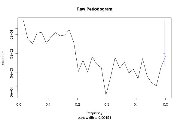
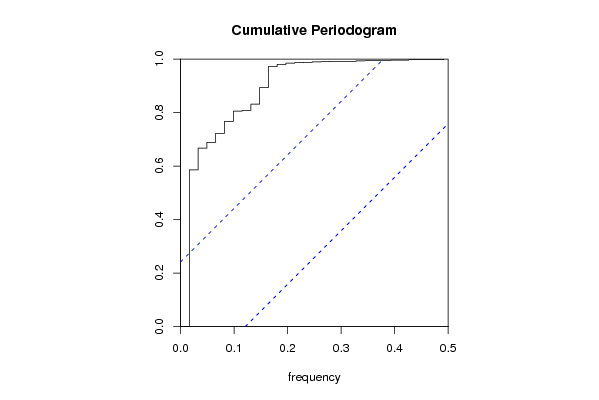
Title produced by software

Spectral Analysis

Date of computation

Tue, 09 Dec 2008 09:01:45 -0700

Cite this page as follows

Statistical Computations at FreeStatistics.org, Office for Research Development and Education, URL https://freestatistics.org/blog/index.php?v=date/2008/Dec/09/t12288385522dwpb0xkxgv4qwh.htm/, Retrieved Fri, 17 May 2024 06:18:05 +0000

Statistical Computations at FreeStatistics.org, Office for Research Development and Education, URL https://freestatistics.org/blog/index.php?pk=31545, Retrieved Fri, 17 May 2024 06:18:05 +0000

QR Codes:

Paste this QR Code to cite your computation.

Original text written by user:

IsPrivate?

No (this computation is public)

User-defined keywords

arma processen WS5 Q2: Spectral analys totaal

Estimated Impact

190

Family? (F = Feedback message, R = changed R code, M = changed R Module, P = changed Parameters, D = changed Data)

F     [Law of Averages] [Random Walk Simul...] [2008-11-25 18:31:28] [b98453cac15ba1066b407e146608df68]
F RM D  [(Partial) Autocorrelation Function] [non stationary ti...] [2008-12-02 20:37:52] [47f64d63202c1921bd27f3073f07a153]
F    D    [(Partial) Autocorrelation Function] [non stationary ti...] [2008-12-02 20:40:11] [47f64d63202c1921bd27f3073f07a153]
-           [(Partial) Autocorrelation Function] [non stationary ti...] [2008-12-02 20:41:59] [47f64d63202c1921bd27f3073f07a153]
F RM          [Variance Reduction Matrix] [non stationary ti...] [2008-12-02 20:44:40] [47f64d63202c1921bd27f3073f07a153]
F   P           [Variance Reduction Matrix] [ARMA proces WS5 Q...] [2008-12-08 20:31:01] [47f64d63202c1921bd27f3073f07a153]
F RMP             [(Partial) Autocorrelation Function] [arma processen WS...] [2008-12-09 15:55:54] [47f64d63202c1921bd27f3073f07a153]
F RMP                 [Spectral Analysis] [arma processen WS...] [2008-12-09 16:01:45] [74c7506a1ea162af3aa8be25bcd05d28] [Current]

Feedback Forum

2008-12-11 11:18:01 [72e979bcc364082694890d2eccc1a66f] [reply] 
Bij de spectraal analyse wordt hetzelfde waargenomen als bij de autocorrelatie functie. In het cumulatief periodogram zie je een duidelijke trend en de trappen wijzen op seizoenaliteit. Dit moet dus weggewerkt worden om tot een stationaire trend te komen.

Post a new message

Dataseries X:

Download CSV

Histogram

Boxplots

8.4
8.4
8.4
8.6
8.9
8.8
8.3
7.5
7.2
7.5
8.8
9.3
9.3
8.7
8.2
8.3
8.5
8.6
8.6
8.2
8.1
8
8.6
8.7
8.8
8.5
8.4
8.5
8.7
8.7
8.6
8.5
8.3
8.1
8.2
8.1
8.1
7.9
7.9
7.9
8
8
7.9
8
7.7
7.2
7.5
7.3
7
7
7
7.2
7.3
7.1
6.8
6.6
6.2
6.2
6.8
6.9
6.8

Summary of computational transaction
Raw Input	view raw input (R code)
Raw Output	view raw output of R engine
Computing time	1 seconds
R Server	'Gwilym Jenkins' @ 72.249.127.135

\begin{tabular}{lllllllll}
\hline
Summary of computational transaction \tabularnewline
Raw Input & view raw input (R code)  \tabularnewline
Raw Output & view raw output of R engine  \tabularnewline
Computing time & 1 seconds \tabularnewline
R Server & 'Gwilym Jenkins' @ 72.249.127.135 \tabularnewline
\hline
\end{tabular}
%Source: https://freestatistics.org/blog/index.php?pk=31545&T=0

[TABLE]
[ROW][C]Summary of computational transaction[/C][/ROW]
[ROW][C]Raw Input[/C][C]view raw input (R code) [/C][/ROW]
[ROW][C]Raw Output[/C][C]view raw output of R engine [/C][/ROW]
[ROW][C]Computing time[/C][C]1 seconds[/C][/ROW]
[ROW][C]R Server[/C][C]'Gwilym Jenkins' @ 72.249.127.135[/C][/ROW]
[/TABLE]
Source: https://freestatistics.org/blog/index.php?pk=31545&T=0

Globally Unique Identifier (entire table): ba.freestatistics.org/blog/index.php?pk=31545&T=0

As an alternative you can also use a QR Code:

The GUIDs for individual cells are displayed in the table below:

Summary of computational transaction
Raw Input	view raw input (R code)
Raw Output	view raw output of R engine
Computing time	1 seconds
R Server	'Gwilym Jenkins' @ 72.249.127.135

Raw Periodogram
Parameter	Value
Box-Cox transformation parameter (lambda)	1
Degree of non-seasonal differencing (d)	0
Degree of seasonal differencing (D)	0
Seasonal Period (s)	12
Frequency (Period)	Spectrum
0.0156 (64)	2.6211
0.0312 (32)	0.271061
0.0469 (21.3333)	0.170108
0.0625 (16)	0.589713
0.0781 (12.8)	0.646404
0.0938 (10.6667)	0.173748
0.1094 (9.1429)	0.356344
0.125 (8)	0.624182
0.1406 (7.1111)	0.423412
0.1562 (6.4)	0.464223
0.1719 (5.8182)	0.870571
0.1875 (5.3333)	0.186909
0.2031 (4.9231)	0.005898
0.2188 (4.5714)	0.022514
0.2344 (4.2667)	0.005501
0.25 (4)	0.034042
0.2656 (3.7647)	0.014028
0.2812 (3.5556)	0.009225
0.2969 (3.3684)	0.000349
0.3125 (3.2)	0.002876
0.3281 (3.0476)	0.031324
0.3438 (2.9091)	0.008649
0.3594 (2.7826)	0.01801
0.375 (2.6667)	0.004944
0.3906 (2.56)	0.007739
0.4062 (2.4615)	0.002492
0.4219 (2.3704)	0.027434
0.4375 (2.2857)	0.003297
0.4531 (2.2069)	0.001504
0.4688 (2.1333)	0.001064
0.4844 (2.0645)	0.009627
0.5 (2)	0.035056

\begin{tabular}{lllllllll}
\hline
Raw Periodogram \tabularnewline
Parameter & Value \tabularnewline
Box-Cox transformation parameter (lambda) & 1 \tabularnewline
Degree of non-seasonal differencing (d) & 0 \tabularnewline
Degree of seasonal differencing (D) & 0 \tabularnewline
Seasonal Period (s) & 12 \tabularnewline
Frequency (Period) & Spectrum \tabularnewline
0.0156 (64) & 2.6211 \tabularnewline
0.0312 (32) & 0.271061 \tabularnewline
0.0469 (21.3333) & 0.170108 \tabularnewline
0.0625 (16) & 0.589713 \tabularnewline
0.0781 (12.8) & 0.646404 \tabularnewline
0.0938 (10.6667) & 0.173748 \tabularnewline
0.1094 (9.1429) & 0.356344 \tabularnewline
0.125 (8) & 0.624182 \tabularnewline
0.1406 (7.1111) & 0.423412 \tabularnewline
0.1562 (6.4) & 0.464223 \tabularnewline
0.1719 (5.8182) & 0.870571 \tabularnewline
0.1875 (5.3333) & 0.186909 \tabularnewline
0.2031 (4.9231) & 0.005898 \tabularnewline
0.2188 (4.5714) & 0.022514 \tabularnewline
0.2344 (4.2667) & 0.005501 \tabularnewline
0.25 (4) & 0.034042 \tabularnewline
0.2656 (3.7647) & 0.014028 \tabularnewline
0.2812 (3.5556) & 0.009225 \tabularnewline
0.2969 (3.3684) & 0.000349 \tabularnewline
0.3125 (3.2) & 0.002876 \tabularnewline
0.3281 (3.0476) & 0.031324 \tabularnewline
0.3438 (2.9091) & 0.008649 \tabularnewline
0.3594 (2.7826) & 0.01801 \tabularnewline
0.375 (2.6667) & 0.004944 \tabularnewline
0.3906 (2.56) & 0.007739 \tabularnewline
0.4062 (2.4615) & 0.002492 \tabularnewline
0.4219 (2.3704) & 0.027434 \tabularnewline
0.4375 (2.2857) & 0.003297 \tabularnewline
0.4531 (2.2069) & 0.001504 \tabularnewline
0.4688 (2.1333) & 0.001064 \tabularnewline
0.4844 (2.0645) & 0.009627 \tabularnewline
0.5 (2) & 0.035056 \tabularnewline
\hline
\end{tabular}
%Source: https://freestatistics.org/blog/index.php?pk=31545&T=1

[TABLE]
[ROW][C]Raw Periodogram[/C][/ROW]
[ROW][C]Parameter[/C][C]Value[/C][/ROW]
[ROW][C]Box-Cox transformation parameter (lambda)[/C][C]1[/C][/ROW]
[ROW][C]Degree of non-seasonal differencing (d)[/C][C]0[/C][/ROW]
[ROW][C]Degree of seasonal differencing (D)[/C][C]0[/C][/ROW]
[ROW][C]Seasonal Period (s)[/C][C]12[/C][/ROW]
[ROW][C]Frequency (Period)[/C][C]Spectrum[/C][/ROW]
[ROW][C]0.0156 (64)[/C][C]2.6211[/C][/ROW]
[ROW][C]0.0312 (32)[/C][C]0.271061[/C][/ROW]
[ROW][C]0.0469 (21.3333)[/C][C]0.170108[/C][/ROW]
[ROW][C]0.0625 (16)[/C][C]0.589713[/C][/ROW]
[ROW][C]0.0781 (12.8)[/C][C]0.646404[/C][/ROW]
[ROW][C]0.0938 (10.6667)[/C][C]0.173748[/C][/ROW]
[ROW][C]0.1094 (9.1429)[/C][C]0.356344[/C][/ROW]
[ROW][C]0.125 (8)[/C][C]0.624182[/C][/ROW]
[ROW][C]0.1406 (7.1111)[/C][C]0.423412[/C][/ROW]
[ROW][C]0.1562 (6.4)[/C][C]0.464223[/C][/ROW]
[ROW][C]0.1719 (5.8182)[/C][C]0.870571[/C][/ROW]
[ROW][C]0.1875 (5.3333)[/C][C]0.186909[/C][/ROW]
[ROW][C]0.2031 (4.9231)[/C][C]0.005898[/C][/ROW]
[ROW][C]0.2188 (4.5714)[/C][C]0.022514[/C][/ROW]
[ROW][C]0.2344 (4.2667)[/C][C]0.005501[/C][/ROW]
[ROW][C]0.25 (4)[/C][C]0.034042[/C][/ROW]
[ROW][C]0.2656 (3.7647)[/C][C]0.014028[/C][/ROW]
[ROW][C]0.2812 (3.5556)[/C][C]0.009225[/C][/ROW]
[ROW][C]0.2969 (3.3684)[/C][C]0.000349[/C][/ROW]
[ROW][C]0.3125 (3.2)[/C][C]0.002876[/C][/ROW]
[ROW][C]0.3281 (3.0476)[/C][C]0.031324[/C][/ROW]
[ROW][C]0.3438 (2.9091)[/C][C]0.008649[/C][/ROW]
[ROW][C]0.3594 (2.7826)[/C][C]0.01801[/C][/ROW]
[ROW][C]0.375 (2.6667)[/C][C]0.004944[/C][/ROW]
[ROW][C]0.3906 (2.56)[/C][C]0.007739[/C][/ROW]
[ROW][C]0.4062 (2.4615)[/C][C]0.002492[/C][/ROW]
[ROW][C]0.4219 (2.3704)[/C][C]0.027434[/C][/ROW]
[ROW][C]0.4375 (2.2857)[/C][C]0.003297[/C][/ROW]
[ROW][C]0.4531 (2.2069)[/C][C]0.001504[/C][/ROW]
[ROW][C]0.4688 (2.1333)[/C][C]0.001064[/C][/ROW]
[ROW][C]0.4844 (2.0645)[/C][C]0.009627[/C][/ROW]
[ROW][C]0.5 (2)[/C][C]0.035056[/C][/ROW]
[/TABLE]
Source: https://freestatistics.org/blog/index.php?pk=31545&T=1

Globally Unique Identifier (entire table): ba.freestatistics.org/blog/index.php?pk=31545&T=1

As an alternative you can also use a QR Code:

The GUIDs for individual cells are displayed in the table below:

Raw Periodogram
Parameter	Value
Box-Cox transformation parameter (lambda)	1
Degree of non-seasonal differencing (d)	0
Degree of seasonal differencing (D)	0
Seasonal Period (s)	12
Frequency (Period)	Spectrum
0.0156 (64)	2.6211
0.0312 (32)	0.271061
0.0469 (21.3333)	0.170108
0.0625 (16)	0.589713
0.0781 (12.8)	0.646404
0.0938 (10.6667)	0.173748
0.1094 (9.1429)	0.356344
0.125 (8)	0.624182
0.1406 (7.1111)	0.423412
0.1562 (6.4)	0.464223
0.1719 (5.8182)	0.870571
0.1875 (5.3333)	0.186909
0.2031 (4.9231)	0.005898
0.2188 (4.5714)	0.022514
0.2344 (4.2667)	0.005501
0.25 (4)	0.034042
0.2656 (3.7647)	0.014028
0.2812 (3.5556)	0.009225
0.2969 (3.3684)	0.000349
0.3125 (3.2)	0.002876
0.3281 (3.0476)	0.031324
0.3438 (2.9091)	0.008649
0.3594 (2.7826)	0.01801
0.375 (2.6667)	0.004944
0.3906 (2.56)	0.007739
0.4062 (2.4615)	0.002492
0.4219 (2.3704)	0.027434
0.4375 (2.2857)	0.003297
0.4531 (2.2069)	0.001504
0.4688 (2.1333)	0.001064
0.4844 (2.0645)	0.009627
0.5 (2)	0.035056

Figure 1

PNG link

Postscript link

PDF link

Figure 2

PNG link

Postscript link

PDF link

Parameters (Session):

par1 = 1 ; par2 = 0 ; par3 = 0 ; par4 = 12 ;

Parameters (R input):

par1 = 1 ; par2 = 0 ; par3 = 0 ; par4 = 12 ;

R code (references can be found in the software module):

par1 <- as.numeric(par1)
par2 <- as.numeric(par2)
par3 <- as.numeric(par3)
par4 <- as.numeric(par4)
if (par1 == 0) {
x <- log(x)
} else {
x <- (x ^ par1 - 1) / par1
}
if (par2 > 0) x <- diff(x,lag=1,difference=par2)
if (par3 > 0) x <- diff(x,lag=par4,difference=par3)
bitmap(file='test1.png')
r <- spectrum(x,main='Raw Periodogram')
dev.off()
bitmap(file='test2.png')
cpgram(x,main='Cumulative Periodogram')
dev.off()
load(file='createtable')
a<-table.start()
a<-table.row.start(a)
a<-table.element(a,'Raw Periodogram',2,TRUE)
a<-table.row.end(a)
a<-table.row.start(a)
a<-table.element(a,'Parameter',header=TRUE)
a<-table.element(a,'Value',header=TRUE)
a<-table.row.end(a)
a<-table.row.start(a)
a<-table.element(a,'Box-Cox transformation parameter (lambda)',header=TRUE)
a<-table.element(a,par1)
a<-table.row.end(a)
a<-table.row.start(a)
a<-table.element(a,'Degree of non-seasonal differencing (d)',header=TRUE)
a<-table.element(a,par2)
a<-table.row.end(a)
a<-table.row.start(a)
a<-table.element(a,'Degree of seasonal differencing (D)',header=TRUE)
a<-table.element(a,par3)
a<-table.row.end(a)
a<-table.row.start(a)
a<-table.element(a,'Seasonal Period (s)',header=TRUE)
a<-table.element(a,par4)
a<-table.row.end(a)
a<-table.row.start(a)
a<-table.element(a,'Frequency (Period)',header=TRUE)
a<-table.element(a,'Spectrum',header=TRUE)
a<-table.row.end(a)
for (i in 1:length(r$freq)) {
a<-table.row.start(a)
mylab <- round(r$freq[i],4)
mylab <- paste(mylab,' (',sep='')
mylab <- paste(mylab,round(1/r$freq[i],4),sep='')
mylab <- paste(mylab,')',sep='')
a<-table.element(a,mylab,header=TRUE)
a<-table.element(a,round(r$spec[i],6))
a<-table.row.end(a)
}
a<-table.end(a)
table.save(a,file='mytable.tab')

Free Statistics

Description of Statistical Computation

Tree of Dependent Computations

Dataset

Tables (Output of Computation)

Figures (Output of Computation)

Input Parameters & R Code