Repository of Reproducible Computations

Free Statistics

of Irreproducible Research!

Author's title

Author

*The author of this computation has been verified*

R Software Module

rwasp_autocorrelation.wasp

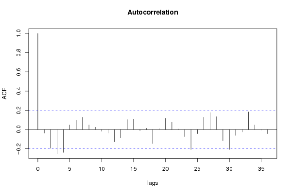
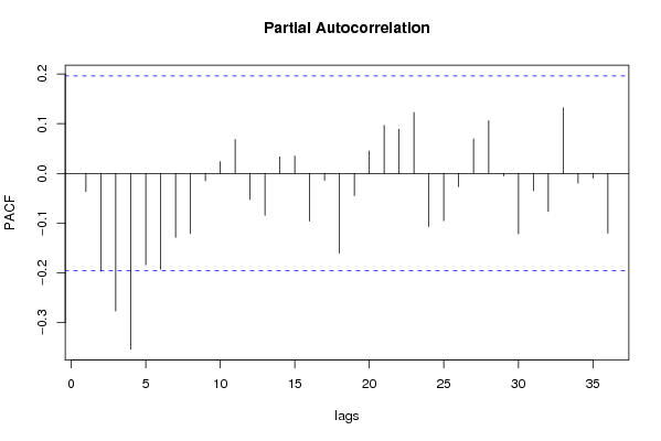
Title produced by software

(Partial) Autocorrelation Function

Date of computation

Sat, 06 Dec 2008 08:51:06 -0700

Cite this page as follows

Statistical Computations at FreeStatistics.org, Office for Research Development and Education, URL https://freestatistics.org/blog/index.php?v=date/2008/Dec/06/t1228578705031gd17ruksjwae.htm/, Retrieved Fri, 17 May 2024 05:14:44 +0000

Statistical Computations at FreeStatistics.org, Office for Research Development and Education, URL https://freestatistics.org/blog/index.php?pk=29714, Retrieved Fri, 17 May 2024 05:14:44 +0000

QR Codes:

Paste this QR Code to cite your computation.

Original text written by user:

IsPrivate?

No (this computation is public)

User-defined keywords

Estimated Impact

219

Family? (F = Feedback message, R = changed R code, M = changed R Module, P = changed Parameters, D = changed Data)

-     [Univariate Data Series] [data set] [2008-12-01 19:54:57] [b98453cac15ba1066b407e146608df68]
F RMP   [(Partial) Autocorrelation Function] [Identification an...] [2008-12-04 19:44:00] [063e4b67ad7d3a8a83eccec794cd5aa7]
F   P     [(Partial) Autocorrelation Function] [Identification an...] [2008-12-04 19:46:29] [063e4b67ad7d3a8a83eccec794cd5aa7]
F   PD      [(Partial) Autocorrelation Function] [Eigen tijdreeks t...] [2008-12-06 15:15:38] [063e4b67ad7d3a8a83eccec794cd5aa7]
F    D        [(Partial) Autocorrelation Function] [Eigen tijdreeks t...] [2008-12-06 15:18:20] [063e4b67ad7d3a8a83eccec794cd5aa7]
-    D            [(Partial) Autocorrelation Function] [Eigen tijdreeks t...] [2008-12-06 15:51:06] [6797a1f4a60918966297e9d9220cabc2] [Current]

Feedback Forum

Post a new message

Dataseries X:

Download CSV

Histogram

Boxplots

6.2
6.1
5.9
5.6
5.5
5.5
5.6
5.7
5.6
5.4
5.3
5.3
5.4
5.5
5.6
5.7
5.8
5.8
5.7
5.9
6.1
6.4
6.4
6.3
6.2
6.2
6.3
6.5
6.6
6.6
6.7
6.6
6.7
7
7.2
7.3
7.5
7.6
7.7
7.8
7.8
7.7
7.6
7.6
7.7
7.8
7.8
7.8
7.7
7.6
7.4
7.1
7.1
7.3
7.6
7.8
7.7
7.6
7.5
7.5
7.5
7.6
7.6
7.7
7.8
7.7
7.6
7.6
7.6
7.7
7.8
7.8
7.9
7.9
7.8
7.8
7.7
7.5
7.1
6.9
7.1
7.1
7.1
7
6.9
6.8
6.7
6.8
6.8
6.7
6.8
6.7
6.6
6.4
6.4
6.4
6.5
6.5
6.4
6.3
6.2
6.3

Summary of computational transaction
Raw Input	view raw input (R code)
Raw Output	view raw output of R engine
Computing time	1 seconds
R Server	'George Udny Yule' @ 72.249.76.132

\begin{tabular}{lllllllll}
\hline
Summary of computational transaction \tabularnewline
Raw Input & view raw input (R code)  \tabularnewline
Raw Output & view raw output of R engine  \tabularnewline
Computing time & 1 seconds \tabularnewline
R Server & 'George Udny Yule' @ 72.249.76.132 \tabularnewline
\hline
\end{tabular}
%Source: https://freestatistics.org/blog/index.php?pk=29714&T=0

[TABLE]
[ROW][C]Summary of computational transaction[/C][/ROW]
[ROW][C]Raw Input[/C][C]view raw input (R code) [/C][/ROW]
[ROW][C]Raw Output[/C][C]view raw output of R engine [/C][/ROW]
[ROW][C]Computing time[/C][C]1 seconds[/C][/ROW]
[ROW][C]R Server[/C][C]'George Udny Yule' @ 72.249.76.132[/C][/ROW]
[/TABLE]
Source: https://freestatistics.org/blog/index.php?pk=29714&T=0

Globally Unique Identifier (entire table): ba.freestatistics.org/blog/index.php?pk=29714&T=0

As an alternative you can also use a QR Code:

The GUIDs for individual cells are displayed in the table below:

Summary of computational transaction
Raw Input	view raw input (R code)
Raw Output	view raw output of R engine
Computing time	1 seconds
R Server	'George Udny Yule' @ 72.249.76.132

Autocorrelation Function
Time lag k	ACF(k)	T-STAT	P-value
1	-0.036719	-0.3672	0.357128
2	-0.195418	-1.9542	0.026736
3	-0.250068	-2.5007	0.00701
4	-0.237873	-2.3787	0.009636
5	0.04878	0.4878	0.313379
6	0.097692	0.9769	0.165483
7	0.127941	1.2794	0.101857
8	0.048773	0.4877	0.313405
9	0.024374	0.2437	0.403965
10	-0.0182	-0.182	0.427977
11	-0.036621	-0.3662	0.357491
12	-0.127865	-1.2787	0.101989
13	-0.085296	-0.853	0.197859
14	0.10365	1.0365	0.151235
15	0.10999	1.0999	0.137008
16	-0.012115	-0.1212	0.451907
17	0.012157	0.1216	0.451743
18	-0.146055	-1.4606	0.073637
19	0.012396	0.124	0.450799
20	0.116199	1.162	0.124003
21	0.078992	0.7899	0.215721
22	0.006167	0.0617	0.475473
23	-0.072879	-0.7288	0.233918
24	-0.207182	-2.0718	0.020428
25	-0.04251	-0.4251	0.335837
26	0.128261	1.2826	0.101298
27	0.177051	1.7705	0.039845
28	0.134111	1.3411	0.091462
29	-0.115953	-1.1595	0.124501
30	-0.207563	-2.0756	0.020247
31	-0.061066	-0.6107	0.271405
32	-0.02423	-0.2423	0.404521
33	0.183135	1.8313	0.035013
34	0.048831	0.4883	0.313198
35	-0.005818	-0.0582	0.476859
36	-0.042537	-0.4254	0.33574

\begin{tabular}{lllllllll}
\hline
Autocorrelation Function \tabularnewline
Time lag k & ACF(k) & T-STAT & P-value \tabularnewline
1 & -0.036719 & -0.3672 & 0.357128 \tabularnewline
2 & -0.195418 & -1.9542 & 0.026736 \tabularnewline
3 & -0.250068 & -2.5007 & 0.00701 \tabularnewline
4 & -0.237873 & -2.3787 & 0.009636 \tabularnewline
5 & 0.04878 & 0.4878 & 0.313379 \tabularnewline
6 & 0.097692 & 0.9769 & 0.165483 \tabularnewline
7 & 0.127941 & 1.2794 & 0.101857 \tabularnewline
8 & 0.048773 & 0.4877 & 0.313405 \tabularnewline
9 & 0.024374 & 0.2437 & 0.403965 \tabularnewline
10 & -0.0182 & -0.182 & 0.427977 \tabularnewline
11 & -0.036621 & -0.3662 & 0.357491 \tabularnewline
12 & -0.127865 & -1.2787 & 0.101989 \tabularnewline
13 & -0.085296 & -0.853 & 0.197859 \tabularnewline
14 & 0.10365 & 1.0365 & 0.151235 \tabularnewline
15 & 0.10999 & 1.0999 & 0.137008 \tabularnewline
16 & -0.012115 & -0.1212 & 0.451907 \tabularnewline
17 & 0.012157 & 0.1216 & 0.451743 \tabularnewline
18 & -0.146055 & -1.4606 & 0.073637 \tabularnewline
19 & 0.012396 & 0.124 & 0.450799 \tabularnewline
20 & 0.116199 & 1.162 & 0.124003 \tabularnewline
21 & 0.078992 & 0.7899 & 0.215721 \tabularnewline
22 & 0.006167 & 0.0617 & 0.475473 \tabularnewline
23 & -0.072879 & -0.7288 & 0.233918 \tabularnewline
24 & -0.207182 & -2.0718 & 0.020428 \tabularnewline
25 & -0.04251 & -0.4251 & 0.335837 \tabularnewline
26 & 0.128261 & 1.2826 & 0.101298 \tabularnewline
27 & 0.177051 & 1.7705 & 0.039845 \tabularnewline
28 & 0.134111 & 1.3411 & 0.091462 \tabularnewline
29 & -0.115953 & -1.1595 & 0.124501 \tabularnewline
30 & -0.207563 & -2.0756 & 0.020247 \tabularnewline
31 & -0.061066 & -0.6107 & 0.271405 \tabularnewline
32 & -0.02423 & -0.2423 & 0.404521 \tabularnewline
33 & 0.183135 & 1.8313 & 0.035013 \tabularnewline
34 & 0.048831 & 0.4883 & 0.313198 \tabularnewline
35 & -0.005818 & -0.0582 & 0.476859 \tabularnewline
36 & -0.042537 & -0.4254 & 0.33574 \tabularnewline
\hline
\end{tabular}
%Source: https://freestatistics.org/blog/index.php?pk=29714&T=1

[TABLE]
[ROW][C]Autocorrelation Function[/C][/ROW]
[ROW][C]Time lag k[/C][C]ACF(k)[/C][C]T-STAT[/C][C]P-value[/C][/ROW]
[ROW][C]1[/C][C]-0.036719[/C][C]-0.3672[/C][C]0.357128[/C][/ROW]
[ROW][C]2[/C][C]-0.195418[/C][C]-1.9542[/C][C]0.026736[/C][/ROW]
[ROW][C]3[/C][C]-0.250068[/C][C]-2.5007[/C][C]0.00701[/C][/ROW]
[ROW][C]4[/C][C]-0.237873[/C][C]-2.3787[/C][C]0.009636[/C][/ROW]
[ROW][C]5[/C][C]0.04878[/C][C]0.4878[/C][C]0.313379[/C][/ROW]
[ROW][C]6[/C][C]0.097692[/C][C]0.9769[/C][C]0.165483[/C][/ROW]
[ROW][C]7[/C][C]0.127941[/C][C]1.2794[/C][C]0.101857[/C][/ROW]
[ROW][C]8[/C][C]0.048773[/C][C]0.4877[/C][C]0.313405[/C][/ROW]
[ROW][C]9[/C][C]0.024374[/C][C]0.2437[/C][C]0.403965[/C][/ROW]
[ROW][C]10[/C][C]-0.0182[/C][C]-0.182[/C][C]0.427977[/C][/ROW]
[ROW][C]11[/C][C]-0.036621[/C][C]-0.3662[/C][C]0.357491[/C][/ROW]
[ROW][C]12[/C][C]-0.127865[/C][C]-1.2787[/C][C]0.101989[/C][/ROW]
[ROW][C]13[/C][C]-0.085296[/C][C]-0.853[/C][C]0.197859[/C][/ROW]
[ROW][C]14[/C][C]0.10365[/C][C]1.0365[/C][C]0.151235[/C][/ROW]
[ROW][C]15[/C][C]0.10999[/C][C]1.0999[/C][C]0.137008[/C][/ROW]
[ROW][C]16[/C][C]-0.012115[/C][C]-0.1212[/C][C]0.451907[/C][/ROW]
[ROW][C]17[/C][C]0.012157[/C][C]0.1216[/C][C]0.451743[/C][/ROW]
[ROW][C]18[/C][C]-0.146055[/C][C]-1.4606[/C][C]0.073637[/C][/ROW]
[ROW][C]19[/C][C]0.012396[/C][C]0.124[/C][C]0.450799[/C][/ROW]
[ROW][C]20[/C][C]0.116199[/C][C]1.162[/C][C]0.124003[/C][/ROW]
[ROW][C]21[/C][C]0.078992[/C][C]0.7899[/C][C]0.215721[/C][/ROW]
[ROW][C]22[/C][C]0.006167[/C][C]0.0617[/C][C]0.475473[/C][/ROW]
[ROW][C]23[/C][C]-0.072879[/C][C]-0.7288[/C][C]0.233918[/C][/ROW]
[ROW][C]24[/C][C]-0.207182[/C][C]-2.0718[/C][C]0.020428[/C][/ROW]
[ROW][C]25[/C][C]-0.04251[/C][C]-0.4251[/C][C]0.335837[/C][/ROW]
[ROW][C]26[/C][C]0.128261[/C][C]1.2826[/C][C]0.101298[/C][/ROW]
[ROW][C]27[/C][C]0.177051[/C][C]1.7705[/C][C]0.039845[/C][/ROW]
[ROW][C]28[/C][C]0.134111[/C][C]1.3411[/C][C]0.091462[/C][/ROW]
[ROW][C]29[/C][C]-0.115953[/C][C]-1.1595[/C][C]0.124501[/C][/ROW]
[ROW][C]30[/C][C]-0.207563[/C][C]-2.0756[/C][C]0.020247[/C][/ROW]
[ROW][C]31[/C][C]-0.061066[/C][C]-0.6107[/C][C]0.271405[/C][/ROW]
[ROW][C]32[/C][C]-0.02423[/C][C]-0.2423[/C][C]0.404521[/C][/ROW]
[ROW][C]33[/C][C]0.183135[/C][C]1.8313[/C][C]0.035013[/C][/ROW]
[ROW][C]34[/C][C]0.048831[/C][C]0.4883[/C][C]0.313198[/C][/ROW]
[ROW][C]35[/C][C]-0.005818[/C][C]-0.0582[/C][C]0.476859[/C][/ROW]
[ROW][C]36[/C][C]-0.042537[/C][C]-0.4254[/C][C]0.33574[/C][/ROW]
[/TABLE]
Source: https://freestatistics.org/blog/index.php?pk=29714&T=1

Globally Unique Identifier (entire table): ba.freestatistics.org/blog/index.php?pk=29714&T=1

As an alternative you can also use a QR Code:

The GUIDs for individual cells are displayed in the table below:

Autocorrelation Function
Time lag k	ACF(k)	T-STAT	P-value
1	-0.036719	-0.3672	0.357128
2	-0.195418	-1.9542	0.026736
3	-0.250068	-2.5007	0.00701
4	-0.237873	-2.3787	0.009636
5	0.04878	0.4878	0.313379
6	0.097692	0.9769	0.165483
7	0.127941	1.2794	0.101857
8	0.048773	0.4877	0.313405
9	0.024374	0.2437	0.403965
10	-0.0182	-0.182	0.427977
11	-0.036621	-0.3662	0.357491
12	-0.127865	-1.2787	0.101989
13	-0.085296	-0.853	0.197859
14	0.10365	1.0365	0.151235
15	0.10999	1.0999	0.137008
16	-0.012115	-0.1212	0.451907
17	0.012157	0.1216	0.451743
18	-0.146055	-1.4606	0.073637
19	0.012396	0.124	0.450799
20	0.116199	1.162	0.124003
21	0.078992	0.7899	0.215721
22	0.006167	0.0617	0.475473
23	-0.072879	-0.7288	0.233918
24	-0.207182	-2.0718	0.020428
25	-0.04251	-0.4251	0.335837
26	0.128261	1.2826	0.101298
27	0.177051	1.7705	0.039845
28	0.134111	1.3411	0.091462
29	-0.115953	-1.1595	0.124501
30	-0.207563	-2.0756	0.020247
31	-0.061066	-0.6107	0.271405
32	-0.02423	-0.2423	0.404521
33	0.183135	1.8313	0.035013
34	0.048831	0.4883	0.313198
35	-0.005818	-0.0582	0.476859
36	-0.042537	-0.4254	0.33574

Partial Autocorrelation Function
Time lag k	PACF(k)	T-STAT	P-value
1	-0.036719	-0.3672	0.357128
2	-0.197032	-1.9703	0.025783
3	-0.277005	-2.7701	0.003341
4	-0.353822	-3.5382	0.000306
5	-0.184108	-1.8411	0.034287
6	-0.193025	-1.9302	0.028205
7	-0.128892	-1.2889	0.100199
8	-0.121454	-1.2145	0.113701
9	-0.014878	-0.1488	0.441015
10	0.023721	0.2372	0.406491
11	0.067983	0.6798	0.24909
12	-0.052721	-0.5272	0.299608
13	-0.084557	-0.8456	0.199905
14	0.033212	0.3321	0.370245
15	0.035184	0.3518	0.362849
16	-0.096078	-0.9608	0.169491
17	-0.013898	-0.139	0.444873
18	-0.16063	-1.6063	0.05568
19	-0.044846	-0.4485	0.327395
20	0.045084	0.4508	0.32654
21	0.09678	0.9678	0.167739
22	0.088815	0.8881	0.188296
23	0.122548	1.2255	0.111637
24	-0.107028	-1.0703	0.143536
25	-0.095445	-0.9545	0.171078
26	-0.026771	-0.2677	0.394738
27	0.069429	0.6943	0.244556
28	0.106025	1.0603	0.145791
29	-0.005215	-0.0521	0.479258
30	-0.121757	-1.2176	0.113126
31	-0.034947	-0.3495	0.363737
32	-0.07682	-0.7682	0.222089
33	0.131817	1.3182	0.095229
34	-0.019684	-0.1968	0.422175
35	-0.009626	-0.0963	0.461754
36	-0.120626	-1.2063	0.115281

\begin{tabular}{lllllllll}
\hline
Partial Autocorrelation Function \tabularnewline
Time lag k & PACF(k) & T-STAT & P-value \tabularnewline
1 & -0.036719 & -0.3672 & 0.357128 \tabularnewline
2 & -0.197032 & -1.9703 & 0.025783 \tabularnewline
3 & -0.277005 & -2.7701 & 0.003341 \tabularnewline
4 & -0.353822 & -3.5382 & 0.000306 \tabularnewline
5 & -0.184108 & -1.8411 & 0.034287 \tabularnewline
6 & -0.193025 & -1.9302 & 0.028205 \tabularnewline
7 & -0.128892 & -1.2889 & 0.100199 \tabularnewline
8 & -0.121454 & -1.2145 & 0.113701 \tabularnewline
9 & -0.014878 & -0.1488 & 0.441015 \tabularnewline
10 & 0.023721 & 0.2372 & 0.406491 \tabularnewline
11 & 0.067983 & 0.6798 & 0.24909 \tabularnewline
12 & -0.052721 & -0.5272 & 0.299608 \tabularnewline
13 & -0.084557 & -0.8456 & 0.199905 \tabularnewline
14 & 0.033212 & 0.3321 & 0.370245 \tabularnewline
15 & 0.035184 & 0.3518 & 0.362849 \tabularnewline
16 & -0.096078 & -0.9608 & 0.169491 \tabularnewline
17 & -0.013898 & -0.139 & 0.444873 \tabularnewline
18 & -0.16063 & -1.6063 & 0.05568 \tabularnewline
19 & -0.044846 & -0.4485 & 0.327395 \tabularnewline
20 & 0.045084 & 0.4508 & 0.32654 \tabularnewline
21 & 0.09678 & 0.9678 & 0.167739 \tabularnewline
22 & 0.088815 & 0.8881 & 0.188296 \tabularnewline
23 & 0.122548 & 1.2255 & 0.111637 \tabularnewline
24 & -0.107028 & -1.0703 & 0.143536 \tabularnewline
25 & -0.095445 & -0.9545 & 0.171078 \tabularnewline
26 & -0.026771 & -0.2677 & 0.394738 \tabularnewline
27 & 0.069429 & 0.6943 & 0.244556 \tabularnewline
28 & 0.106025 & 1.0603 & 0.145791 \tabularnewline
29 & -0.005215 & -0.0521 & 0.479258 \tabularnewline
30 & -0.121757 & -1.2176 & 0.113126 \tabularnewline
31 & -0.034947 & -0.3495 & 0.363737 \tabularnewline
32 & -0.07682 & -0.7682 & 0.222089 \tabularnewline
33 & 0.131817 & 1.3182 & 0.095229 \tabularnewline
34 & -0.019684 & -0.1968 & 0.422175 \tabularnewline
35 & -0.009626 & -0.0963 & 0.461754 \tabularnewline
36 & -0.120626 & -1.2063 & 0.115281 \tabularnewline
\hline
\end{tabular}
%Source: https://freestatistics.org/blog/index.php?pk=29714&T=2

[TABLE]
[ROW][C]Partial Autocorrelation Function[/C][/ROW]
[ROW][C]Time lag k[/C][C]PACF(k)[/C][C]T-STAT[/C][C]P-value[/C][/ROW]
[ROW][C]1[/C][C]-0.036719[/C][C]-0.3672[/C][C]0.357128[/C][/ROW]
[ROW][C]2[/C][C]-0.197032[/C][C]-1.9703[/C][C]0.025783[/C][/ROW]
[ROW][C]3[/C][C]-0.277005[/C][C]-2.7701[/C][C]0.003341[/C][/ROW]
[ROW][C]4[/C][C]-0.353822[/C][C]-3.5382[/C][C]0.000306[/C][/ROW]
[ROW][C]5[/C][C]-0.184108[/C][C]-1.8411[/C][C]0.034287[/C][/ROW]
[ROW][C]6[/C][C]-0.193025[/C][C]-1.9302[/C][C]0.028205[/C][/ROW]
[ROW][C]7[/C][C]-0.128892[/C][C]-1.2889[/C][C]0.100199[/C][/ROW]
[ROW][C]8[/C][C]-0.121454[/C][C]-1.2145[/C][C]0.113701[/C][/ROW]
[ROW][C]9[/C][C]-0.014878[/C][C]-0.1488[/C][C]0.441015[/C][/ROW]
[ROW][C]10[/C][C]0.023721[/C][C]0.2372[/C][C]0.406491[/C][/ROW]
[ROW][C]11[/C][C]0.067983[/C][C]0.6798[/C][C]0.24909[/C][/ROW]
[ROW][C]12[/C][C]-0.052721[/C][C]-0.5272[/C][C]0.299608[/C][/ROW]
[ROW][C]13[/C][C]-0.084557[/C][C]-0.8456[/C][C]0.199905[/C][/ROW]
[ROW][C]14[/C][C]0.033212[/C][C]0.3321[/C][C]0.370245[/C][/ROW]
[ROW][C]15[/C][C]0.035184[/C][C]0.3518[/C][C]0.362849[/C][/ROW]
[ROW][C]16[/C][C]-0.096078[/C][C]-0.9608[/C][C]0.169491[/C][/ROW]
[ROW][C]17[/C][C]-0.013898[/C][C]-0.139[/C][C]0.444873[/C][/ROW]
[ROW][C]18[/C][C]-0.16063[/C][C]-1.6063[/C][C]0.05568[/C][/ROW]
[ROW][C]19[/C][C]-0.044846[/C][C]-0.4485[/C][C]0.327395[/C][/ROW]
[ROW][C]20[/C][C]0.045084[/C][C]0.4508[/C][C]0.32654[/C][/ROW]
[ROW][C]21[/C][C]0.09678[/C][C]0.9678[/C][C]0.167739[/C][/ROW]
[ROW][C]22[/C][C]0.088815[/C][C]0.8881[/C][C]0.188296[/C][/ROW]
[ROW][C]23[/C][C]0.122548[/C][C]1.2255[/C][C]0.111637[/C][/ROW]
[ROW][C]24[/C][C]-0.107028[/C][C]-1.0703[/C][C]0.143536[/C][/ROW]
[ROW][C]25[/C][C]-0.095445[/C][C]-0.9545[/C][C]0.171078[/C][/ROW]
[ROW][C]26[/C][C]-0.026771[/C][C]-0.2677[/C][C]0.394738[/C][/ROW]
[ROW][C]27[/C][C]0.069429[/C][C]0.6943[/C][C]0.244556[/C][/ROW]
[ROW][C]28[/C][C]0.106025[/C][C]1.0603[/C][C]0.145791[/C][/ROW]
[ROW][C]29[/C][C]-0.005215[/C][C]-0.0521[/C][C]0.479258[/C][/ROW]
[ROW][C]30[/C][C]-0.121757[/C][C]-1.2176[/C][C]0.113126[/C][/ROW]
[ROW][C]31[/C][C]-0.034947[/C][C]-0.3495[/C][C]0.363737[/C][/ROW]
[ROW][C]32[/C][C]-0.07682[/C][C]-0.7682[/C][C]0.222089[/C][/ROW]
[ROW][C]33[/C][C]0.131817[/C][C]1.3182[/C][C]0.095229[/C][/ROW]
[ROW][C]34[/C][C]-0.019684[/C][C]-0.1968[/C][C]0.422175[/C][/ROW]
[ROW][C]35[/C][C]-0.009626[/C][C]-0.0963[/C][C]0.461754[/C][/ROW]
[ROW][C]36[/C][C]-0.120626[/C][C]-1.2063[/C][C]0.115281[/C][/ROW]
[/TABLE]
Source: https://freestatistics.org/blog/index.php?pk=29714&T=2

Globally Unique Identifier (entire table): ba.freestatistics.org/blog/index.php?pk=29714&T=2

As an alternative you can also use a QR Code:

The GUIDs for individual cells are displayed in the table below:

Partial Autocorrelation Function
Time lag k	PACF(k)	T-STAT	P-value
1	-0.036719	-0.3672	0.357128
2	-0.197032	-1.9703	0.025783
3	-0.277005	-2.7701	0.003341
4	-0.353822	-3.5382	0.000306
5	-0.184108	-1.8411	0.034287
6	-0.193025	-1.9302	0.028205
7	-0.128892	-1.2889	0.100199
8	-0.121454	-1.2145	0.113701
9	-0.014878	-0.1488	0.441015
10	0.023721	0.2372	0.406491
11	0.067983	0.6798	0.24909
12	-0.052721	-0.5272	0.299608
13	-0.084557	-0.8456	0.199905
14	0.033212	0.3321	0.370245
15	0.035184	0.3518	0.362849
16	-0.096078	-0.9608	0.169491
17	-0.013898	-0.139	0.444873
18	-0.16063	-1.6063	0.05568
19	-0.044846	-0.4485	0.327395
20	0.045084	0.4508	0.32654
21	0.09678	0.9678	0.167739
22	0.088815	0.8881	0.188296
23	0.122548	1.2255	0.111637
24	-0.107028	-1.0703	0.143536
25	-0.095445	-0.9545	0.171078
26	-0.026771	-0.2677	0.394738
27	0.069429	0.6943	0.244556
28	0.106025	1.0603	0.145791
29	-0.005215	-0.0521	0.479258
30	-0.121757	-1.2176	0.113126
31	-0.034947	-0.3495	0.363737
32	-0.07682	-0.7682	0.222089
33	0.131817	1.3182	0.095229
34	-0.019684	-0.1968	0.422175
35	-0.009626	-0.0963	0.461754
36	-0.120626	-1.2063	0.115281

Figure 1

PNG link

Postscript link

PDF link

Figure 2

PNG link

Postscript link

PDF link

Parameters (Session):

par1 = 60 ; par2 = 1 ; par3 = 0 ; par4 = 0 ; par5 = 12 ;

Parameters (R input):

par1 = 36 ; par2 = 1 ; par3 = 2 ; par4 = 0 ; par5 = 12 ;

R code (references can be found in the software module):

if (par1 == 'Default') {
par1 = 10*log10(length(x))
} else {
par1 <- as.numeric(par1)
}
par2 <- as.numeric(par2)
par3 <- as.numeric(par3)
par4 <- as.numeric(par4)
par5 <- as.numeric(par5)
if (par2 == 0) {
x <- log(x)
} else {
x <- (x ^ par2 - 1) / par2
}
if (par3 > 0) x <- diff(x,lag=1,difference=par3)
if (par4 > 0) x <- diff(x,lag=par5,difference=par4)
bitmap(file='pic1.png')
racf <- acf(x,par1,main='Autocorrelation',xlab='lags',ylab='ACF')
dev.off()
bitmap(file='pic2.png')
rpacf <- pacf(x,par1,main='Partial Autocorrelation',xlab='lags',ylab='PACF')
dev.off()
(myacf <- c(racf$acf))
(mypacf <- c(rpacf$acf))
lengthx <- length(x)
sqrtn <- sqrt(lengthx)
load(file='createtable')
a<-table.start()
a<-table.row.start(a)
a<-table.element(a,'Autocorrelation Function',4,TRUE)
a<-table.row.end(a)
a<-table.row.start(a)
a<-table.element(a,'Time lag k',header=TRUE)
a<-table.element(a,hyperlink('basics.htm','ACF(k)','click here for more information about the Autocorrelation Function'),header=TRUE)
a<-table.element(a,'T-STAT',header=TRUE)
a<-table.element(a,'P-value',header=TRUE)
a<-table.row.end(a)
for (i in 2:(par1+1)) {
a<-table.row.start(a)
a<-table.element(a,i-1,header=TRUE)
a<-table.element(a,round(myacf[i],6))
mytstat <- myacf[i]*sqrtn
a<-table.element(a,round(mytstat,4))
a<-table.element(a,round(1-pt(abs(mytstat),lengthx),6))
a<-table.row.end(a)
}
a<-table.end(a)
table.save(a,file='mytable.tab')
a<-table.start()
a<-table.row.start(a)
a<-table.element(a,'Partial Autocorrelation Function',4,TRUE)
a<-table.row.end(a)
a<-table.row.start(a)
a<-table.element(a,'Time lag k',header=TRUE)
a<-table.element(a,hyperlink('basics.htm','PACF(k)','click here for more information about the Partial Autocorrelation Function'),header=TRUE)
a<-table.element(a,'T-STAT',header=TRUE)
a<-table.element(a,'P-value',header=TRUE)
a<-table.row.end(a)
for (i in 1:par1) {
a<-table.row.start(a)
a<-table.element(a,i,header=TRUE)
a<-table.element(a,round(mypacf[i],6))
mytstat <- mypacf[i]*sqrtn
a<-table.element(a,round(mytstat,4))
a<-table.element(a,round(1-pt(abs(mytstat),lengthx),6))
a<-table.row.end(a)
}
a<-table.end(a)
table.save(a,file='mytable1.tab')

Free Statistics

Description of Statistical Computation

Tree of Dependent Computations

Dataset

Tables (Output of Computation)

Figures (Output of Computation)

Input Parameters & R Code