Repository of Reproducible Computations

Free Statistics

of Irreproducible Research!

Author's title

Author

*Unverified author*

R Software Module

rwasp_smp.wasp

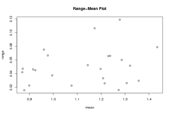
Title produced by software

Standard Deviation-Mean Plot

Date of computation

Wed, 03 Dec 2008 01:44:18 -0700

Cite this page as follows

Statistical Computations at FreeStatistics.org, Office for Research Development and Education, URL https://freestatistics.org/blog/index.php?v=date/2008/Dec/03/t12282939002er0uhq5nzijxk9.htm/, Retrieved Fri, 17 May 2024 05:14:12 +0000

Statistical Computations at FreeStatistics.org, Office for Research Development and Education, URL https://freestatistics.org/blog/index.php?pk=28576, Retrieved Fri, 17 May 2024 05:14:12 +0000

QR Codes:

Paste this QR Code to cite your computation.

Original text written by user:

IsPrivate?

No (this computation is public)

User-defined keywords

Estimated Impact

211

Family? (F = Feedback message, R = changed R code, M = changed R Module, P = changed Parameters, D = changed Data)

F       [Standard Deviation-Mean Plot] [] [2008-12-03 08:44:18] [ee5aee65e0c44ac54c8097a6e28e37f4] [Current]

Feedback Forum

2008-12-08 13:47:38 [Li Tang Hu] [reply] 
we kunnen de lmbdawaarde niet gaan gebruiken omdat beide pwaarden groter zijn dan 0.05.dus gaan we de lambdawaarde op 1 houden.

Post a new message

Dataseries X:

Download CSV

Histogram

Boxplots

Summary of computational transaction
Raw Input	view raw input (R code)
Raw Output	view raw output of R engine
Computing time	1 seconds
R Server	'Gwilym Jenkins' @ 72.249.127.135

\begin{tabular}{lllllllll}
\hline
Summary of computational transaction \tabularnewline
Raw Input & view raw input (R code)  \tabularnewline
Raw Output & view raw output of R engine  \tabularnewline
Computing time & 1 seconds \tabularnewline
R Server & 'Gwilym Jenkins' @ 72.249.127.135 \tabularnewline
\hline
\end{tabular}
%Source: https://freestatistics.org/blog/index.php?pk=28576&T=0

[TABLE]
[ROW][C]Summary of computational transaction[/C][/ROW]
[ROW][C]Raw Input[/C][C]view raw input (R code) [/C][/ROW]
[ROW][C]Raw Output[/C][C]view raw output of R engine [/C][/ROW]
[ROW][C]Computing time[/C][C]1 seconds[/C][/ROW]
[ROW][C]R Server[/C][C]'Gwilym Jenkins' @ 72.249.127.135[/C][/ROW]
[/TABLE]
Source: https://freestatistics.org/blog/index.php?pk=28576&T=0

Globally Unique Identifier (entire table): ba.freestatistics.org/blog/index.php?pk=28576&T=0

As an alternative you can also use a QR Code:

The GUIDs for individual cells are displayed in the table below:

Summary of computational transaction
Raw Input	view raw input (R code)
Raw Output	view raw output of R engine
Computing time	1 seconds
R Server	'Gwilym Jenkins' @ 72.249.127.135

Standard Deviation-Mean Plot
Section	Mean	Standard Deviation	Range
1	0.9771	0.0285721309437478	0.0667000000000001
2	0.92475	0.0230888862153779	0.0451
3	0.87025	0.0196082465644772	0.0421
4	0.915375	0.0195488064426791	0.0463
5	0.87215	0.0208016826242494	0.0473
6	0.899425	0.0108220068995235	0.0228000000000000
7	0.878725	0.0072034135426662	0.0158000000000000
8	0.9606	0.0327739734138742	0.0752
9	0.9954	0.0180560239255491	0.0375
10	1.07625	0.009855793558444	0.0226000000000000
11	1.1439	0.0234601790274499	0.0524
12	1.17255	0.0435640142013259	0.106400000000000
13	1.23765	0.031355222850428	0.0661
14	1.214675	0.0107521703235517	0.0258999999999998
15	1.277675	0.0528774290222208	0.119
16	1.3068	0.0115622950432285	0.0263
17	1.2297	0.0284404641312339	0.0657000000000001
18	1.197825	0.0208487209839517	0.0469999999999999
19	1.2083	0.0142288439446078	0.0333000000000001
20	1.272875	0.00745447293017196	0.0161
21	1.2858	0.0261230421913936	0.0601999999999998
22	1.320775	0.0229242775240573	0.0516999999999999
23	1.3567	0.0129442393879800	0.0296999999999998
24	1.434425	0.0356402745032452	0.0788

\begin{tabular}{lllllllll}
\hline
Standard Deviation-Mean Plot \tabularnewline
Section & Mean & Standard Deviation & Range \tabularnewline
1 & 0.9771 & 0.0285721309437478 & 0.0667000000000001 \tabularnewline
2 & 0.92475 & 0.0230888862153779 & 0.0451 \tabularnewline
3 & 0.87025 & 0.0196082465644772 & 0.0421 \tabularnewline
4 & 0.915375 & 0.0195488064426791 & 0.0463 \tabularnewline
5 & 0.87215 & 0.0208016826242494 & 0.0473 \tabularnewline
6 & 0.899425 & 0.0108220068995235 & 0.0228000000000000 \tabularnewline
7 & 0.878725 & 0.0072034135426662 & 0.0158000000000000 \tabularnewline
8 & 0.9606 & 0.0327739734138742 & 0.0752 \tabularnewline
9 & 0.9954 & 0.0180560239255491 & 0.0375 \tabularnewline
10 & 1.07625 & 0.009855793558444 & 0.0226000000000000 \tabularnewline
11 & 1.1439 & 0.0234601790274499 & 0.0524 \tabularnewline
12 & 1.17255 & 0.0435640142013259 & 0.106400000000000 \tabularnewline
13 & 1.23765 & 0.031355222850428 & 0.0661 \tabularnewline
14 & 1.214675 & 0.0107521703235517 & 0.0258999999999998 \tabularnewline
15 & 1.277675 & 0.0528774290222208 & 0.119 \tabularnewline
16 & 1.3068 & 0.0115622950432285 & 0.0263 \tabularnewline
17 & 1.2297 & 0.0284404641312339 & 0.0657000000000001 \tabularnewline
18 & 1.197825 & 0.0208487209839517 & 0.0469999999999999 \tabularnewline
19 & 1.2083 & 0.0142288439446078 & 0.0333000000000001 \tabularnewline
20 & 1.272875 & 0.00745447293017196 & 0.0161 \tabularnewline
21 & 1.2858 & 0.0261230421913936 & 0.0601999999999998 \tabularnewline
22 & 1.320775 & 0.0229242775240573 & 0.0516999999999999 \tabularnewline
23 & 1.3567 & 0.0129442393879800 & 0.0296999999999998 \tabularnewline
24 & 1.434425 & 0.0356402745032452 & 0.0788 \tabularnewline
\hline
\end{tabular}
%Source: https://freestatistics.org/blog/index.php?pk=28576&T=1

[TABLE]
[ROW][C]Standard Deviation-Mean Plot[/C][/ROW]
[ROW][C]Section[/C][C]Mean[/C][C]Standard Deviation[/C][C]Range[/C][/ROW]
[ROW][C]1[/C][C]0.9771[/C][C]0.0285721309437478[/C][C]0.0667000000000001[/C][/ROW]
[ROW][C]2[/C][C]0.92475[/C][C]0.0230888862153779[/C][C]0.0451[/C][/ROW]
[ROW][C]3[/C][C]0.87025[/C][C]0.0196082465644772[/C][C]0.0421[/C][/ROW]
[ROW][C]4[/C][C]0.915375[/C][C]0.0195488064426791[/C][C]0.0463[/C][/ROW]
[ROW][C]5[/C][C]0.87215[/C][C]0.0208016826242494[/C][C]0.0473[/C][/ROW]
[ROW][C]6[/C][C]0.899425[/C][C]0.0108220068995235[/C][C]0.0228000000000000[/C][/ROW]
[ROW][C]7[/C][C]0.878725[/C][C]0.0072034135426662[/C][C]0.0158000000000000[/C][/ROW]
[ROW][C]8[/C][C]0.9606[/C][C]0.0327739734138742[/C][C]0.0752[/C][/ROW]
[ROW][C]9[/C][C]0.9954[/C][C]0.0180560239255491[/C][C]0.0375[/C][/ROW]
[ROW][C]10[/C][C]1.07625[/C][C]0.009855793558444[/C][C]0.0226000000000000[/C][/ROW]
[ROW][C]11[/C][C]1.1439[/C][C]0.0234601790274499[/C][C]0.0524[/C][/ROW]
[ROW][C]12[/C][C]1.17255[/C][C]0.0435640142013259[/C][C]0.106400000000000[/C][/ROW]
[ROW][C]13[/C][C]1.23765[/C][C]0.031355222850428[/C][C]0.0661[/C][/ROW]
[ROW][C]14[/C][C]1.214675[/C][C]0.0107521703235517[/C][C]0.0258999999999998[/C][/ROW]
[ROW][C]15[/C][C]1.277675[/C][C]0.0528774290222208[/C][C]0.119[/C][/ROW]
[ROW][C]16[/C][C]1.3068[/C][C]0.0115622950432285[/C][C]0.0263[/C][/ROW]
[ROW][C]17[/C][C]1.2297[/C][C]0.0284404641312339[/C][C]0.0657000000000001[/C][/ROW]
[ROW][C]18[/C][C]1.197825[/C][C]0.0208487209839517[/C][C]0.0469999999999999[/C][/ROW]
[ROW][C]19[/C][C]1.2083[/C][C]0.0142288439446078[/C][C]0.0333000000000001[/C][/ROW]
[ROW][C]20[/C][C]1.272875[/C][C]0.00745447293017196[/C][C]0.0161[/C][/ROW]
[ROW][C]21[/C][C]1.2858[/C][C]0.0261230421913936[/C][C]0.0601999999999998[/C][/ROW]
[ROW][C]22[/C][C]1.320775[/C][C]0.0229242775240573[/C][C]0.0516999999999999[/C][/ROW]
[ROW][C]23[/C][C]1.3567[/C][C]0.0129442393879800[/C][C]0.0296999999999998[/C][/ROW]
[ROW][C]24[/C][C]1.434425[/C][C]0.0356402745032452[/C][C]0.0788[/C][/ROW]
[/TABLE]
Source: https://freestatistics.org/blog/index.php?pk=28576&T=1

Globally Unique Identifier (entire table): ba.freestatistics.org/blog/index.php?pk=28576&T=1

As an alternative you can also use a QR Code:

The GUIDs for individual cells are displayed in the table below:

Standard Deviation-Mean Plot
Section	Mean	Standard Deviation	Range
1	0.9771	0.0285721309437478	0.0667000000000001
2	0.92475	0.0230888862153779	0.0451
3	0.87025	0.0196082465644772	0.0421
4	0.915375	0.0195488064426791	0.0463
5	0.87215	0.0208016826242494	0.0473
6	0.899425	0.0108220068995235	0.0228000000000000
7	0.878725	0.0072034135426662	0.0158000000000000
8	0.9606	0.0327739734138742	0.0752
9	0.9954	0.0180560239255491	0.0375
10	1.07625	0.009855793558444	0.0226000000000000
11	1.1439	0.0234601790274499	0.0524
12	1.17255	0.0435640142013259	0.106400000000000
13	1.23765	0.031355222850428	0.0661
14	1.214675	0.0107521703235517	0.0258999999999998
15	1.277675	0.0528774290222208	0.119
16	1.3068	0.0115622950432285	0.0263
17	1.2297	0.0284404641312339	0.0657000000000001
18	1.197825	0.0208487209839517	0.0469999999999999
19	1.2083	0.0142288439446078	0.0333000000000001
20	1.272875	0.00745447293017196	0.0161
21	1.2858	0.0261230421913936	0.0601999999999998
22	1.320775	0.0229242775240573	0.0516999999999999
23	1.3567	0.0129442393879800	0.0296999999999998
24	1.434425	0.0356402745032452	0.0788

Regression: S.E.(k) = alpha + beta * Mean(k)
alpha	0.00615922536338457
beta	0.0142319580784528
S.D.	0.0133740472025242
T-STAT	1.06414743891189
p-value	0.298803025710894

\begin{tabular}{lllllllll}
\hline
Regression: S.E.(k) = alpha + beta * Mean(k) \tabularnewline
alpha & 0.00615922536338457 \tabularnewline
beta & 0.0142319580784528 \tabularnewline
S.D. & 0.0133740472025242 \tabularnewline
T-STAT & 1.06414743891189 \tabularnewline
p-value & 0.298803025710894 \tabularnewline
\hline
\end{tabular}
%Source: https://freestatistics.org/blog/index.php?pk=28576&T=2

[TABLE]
[ROW][C]Regression: S.E.(k) = alpha + beta * Mean(k)[/C][/ROW]
[ROW][C]alpha[/C][C]0.00615922536338457[/C][/ROW]
[ROW][C]beta[/C][C]0.0142319580784528[/C][/ROW]
[ROW][C]S.D.[/C][C]0.0133740472025242[/C][/ROW]
[ROW][C]T-STAT[/C][C]1.06414743891189[/C][/ROW]
[ROW][C]p-value[/C][C]0.298803025710894[/C][/ROW]
[/TABLE]
Source: https://freestatistics.org/blog/index.php?pk=28576&T=2

Globally Unique Identifier (entire table): ba.freestatistics.org/blog/index.php?pk=28576&T=2

As an alternative you can also use a QR Code:

The GUIDs for individual cells are displayed in the table below:

Regression: S.E.(k) = alpha + beta * Mean(k)
alpha	0.00615922536338457
beta	0.0142319580784528
S.D.	0.0133740472025242
T-STAT	1.06414743891189
p-value	0.298803025710894

Regression: ln S.E.(k) = alpha + beta * ln Mean(k)
alpha	-3.99973996699091
beta	0.569372129084798
S.D.	0.692506670390832
T-STAT	0.822190100729947
p-value	0.419790934502606
Lambda	0.430627870915202

\begin{tabular}{lllllllll}
\hline
Regression: ln S.E.(k) = alpha + beta * ln Mean(k) \tabularnewline
alpha & -3.99973996699091 \tabularnewline
beta & 0.569372129084798 \tabularnewline
S.D. & 0.692506670390832 \tabularnewline
T-STAT & 0.822190100729947 \tabularnewline
p-value & 0.419790934502606 \tabularnewline
Lambda & 0.430627870915202 \tabularnewline
\hline
\end{tabular}
%Source: https://freestatistics.org/blog/index.php?pk=28576&T=3

[TABLE]
[ROW][C]Regression: ln S.E.(k) = alpha + beta * ln Mean(k)[/C][/ROW]
[ROW][C]alpha[/C][C]-3.99973996699091[/C][/ROW]
[ROW][C]beta[/C][C]0.569372129084798[/C][/ROW]
[ROW][C]S.D.[/C][C]0.692506670390832[/C][/ROW]
[ROW][C]T-STAT[/C][C]0.822190100729947[/C][/ROW]
[ROW][C]p-value[/C][C]0.419790934502606[/C][/ROW]
[ROW][C]Lambda[/C][C]0.430627870915202[/C][/ROW]
[/TABLE]
Source: https://freestatistics.org/blog/index.php?pk=28576&T=3

Globally Unique Identifier (entire table): ba.freestatistics.org/blog/index.php?pk=28576&T=3

As an alternative you can also use a QR Code:

The GUIDs for individual cells are displayed in the table below:

Regression: ln S.E.(k) = alpha + beta * ln Mean(k)
alpha	-3.99973996699091
beta	0.569372129084798
S.D.	0.692506670390832
T-STAT	0.822190100729947
p-value	0.419790934502606
Lambda	0.430627870915202

Figure 1

PNG link

Postscript link

PDF link

Figure 2

PNG link

Postscript link

PDF link

Parameters (Session):

par1 = 4 ;

Parameters (R input):

par1 = 4 ;

R code (references can be found in the software module):

par1 <- as.numeric(par1)
(n <- length(x))
(np <- floor(n / par1))
arr <- array(NA,dim=c(par1,np))
j <- 0
k <- 1
for (i in 1:(np*par1))
{
j = j + 1
arr[j,k] <- x[i]
if (j == par1) {
j = 0
k=k+1
}
}
arr
arr.mean <- array(NA,dim=np)
arr.sd <- array(NA,dim=np)
arr.range <- array(NA,dim=np)
for (j in 1:np)
{
arr.mean[j] <- mean(arr[,j],na.rm=TRUE)
arr.sd[j] <- sd(arr[,j],na.rm=TRUE)
arr.range[j] <- max(arr[,j],na.rm=TRUE) - min(arr[,j],na.rm=TRUE)
}
arr.mean
arr.sd
arr.range
(lm1 <- lm(arr.sd~arr.mean))
(lnlm1 <- lm(log(arr.sd)~log(arr.mean)))
(lm2 <- lm(arr.range~arr.mean))
bitmap(file='test1.png')
plot(arr.mean,arr.sd,main='Standard Deviation-Mean Plot',xlab='mean',ylab='standard deviation')
dev.off()
bitmap(file='test2.png')
plot(arr.mean,arr.range,main='Range-Mean Plot',xlab='mean',ylab='range')
dev.off()
load(file='createtable')
a<-table.start()
a<-table.row.start(a)
a<-table.element(a,'Standard Deviation-Mean Plot',4,TRUE)
a<-table.row.end(a)
a<-table.row.start(a)
a<-table.element(a,'Section',header=TRUE)
a<-table.element(a,'Mean',header=TRUE)
a<-table.element(a,'Standard Deviation',header=TRUE)
a<-table.element(a,'Range',header=TRUE)
a<-table.row.end(a)
for (j in 1:np) {
a<-table.row.start(a)
a<-table.element(a,j,header=TRUE)
a<-table.element(a,arr.mean[j])
a<-table.element(a,arr.sd[j] )
a<-table.element(a,arr.range[j] )
a<-table.row.end(a)
}
a<-table.end(a)
table.save(a,file='mytable.tab')
a<-table.start()
a<-table.row.start(a)
a<-table.element(a,'Regression: S.E.(k) = alpha + beta * Mean(k)',2,TRUE)
a<-table.row.end(a)
a<-table.row.start(a)
a<-table.element(a,'alpha',header=TRUE)
a<-table.element(a,lm1$coefficients[[1]])
a<-table.row.end(a)
a<-table.row.start(a)
a<-table.element(a,'beta',header=TRUE)
a<-table.element(a,lm1$coefficients[[2]])
a<-table.row.end(a)
a<-table.row.start(a)
a<-table.element(a,'S.D.',header=TRUE)
a<-table.element(a,summary(lm1)$coefficients[2,2])
a<-table.row.end(a)
a<-table.row.start(a)
a<-table.element(a,'T-STAT',header=TRUE)
a<-table.element(a,summary(lm1)$coefficients[2,3])
a<-table.row.end(a)
a<-table.row.start(a)
a<-table.element(a,'p-value',header=TRUE)
a<-table.element(a,summary(lm1)$coefficients[2,4])
a<-table.row.end(a)
a<-table.end(a)
table.save(a,file='mytable1.tab')
a<-table.start()
a<-table.row.start(a)
a<-table.element(a,'Regression: ln S.E.(k) = alpha + beta * ln Mean(k)',2,TRUE)
a<-table.row.end(a)
a<-table.row.start(a)
a<-table.element(a,'alpha',header=TRUE)
a<-table.element(a,lnlm1$coefficients[[1]])
a<-table.row.end(a)
a<-table.row.start(a)
a<-table.element(a,'beta',header=TRUE)
a<-table.element(a,lnlm1$coefficients[[2]])
a<-table.row.end(a)
a<-table.row.start(a)
a<-table.element(a,'S.D.',header=TRUE)
a<-table.element(a,summary(lnlm1)$coefficients[2,2])
a<-table.row.end(a)
a<-table.row.start(a)
a<-table.element(a,'T-STAT',header=TRUE)
a<-table.element(a,summary(lnlm1)$coefficients[2,3])
a<-table.row.end(a)
a<-table.row.start(a)
a<-table.element(a,'p-value',header=TRUE)
a<-table.element(a,summary(lnlm1)$coefficients[2,4])
a<-table.row.end(a)
a<-table.row.start(a)
a<-table.element(a,'Lambda',header=TRUE)
a<-table.element(a,1-lnlm1$coefficients[[2]])
a<-table.row.end(a)
a<-table.end(a)
table.save(a,file='mytable2.tab')

Free Statistics

Description of Statistical Computation

Tree of Dependent Computations

Dataset

Tables (Output of Computation)

Figures (Output of Computation)

Input Parameters & R Code