Repository of Reproducible Computations

Free Statistics

of Irreproducible Research!

Author's title

Author

*The author of this computation has been verified*

R Software Module

rwasp_spectrum.wasp

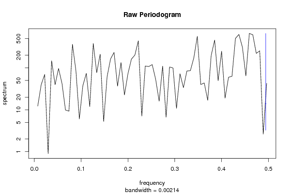
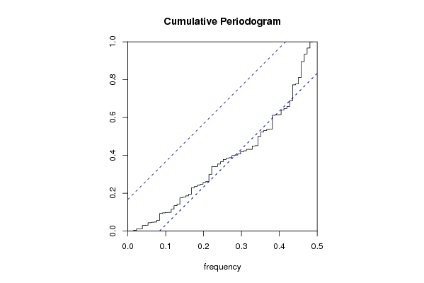
Title produced by software

Spectral Analysis

Date of computation

Tue, 02 Dec 2008 13:56:02 -0700

Cite this page as follows

Statistical Computations at FreeStatistics.org, Office for Research Development and Education, URL https://freestatistics.org/blog/index.php?v=date/2008/Dec/02/t1228251433uycqx3cen3yxn4i.htm/, Retrieved Fri, 17 May 2024 02:02:55 +0000

Statistical Computations at FreeStatistics.org, Office for Research Development and Education, URL https://freestatistics.org/blog/index.php?pk=28448, Retrieved Fri, 17 May 2024 02:02:55 +0000

QR Codes:

Paste this QR Code to cite your computation.

Original text written by user:

IsPrivate?

No (this computation is public)

User-defined keywords

Estimated Impact

189

Family? (F = Feedback message, R = changed R code, M = changed R Module, P = changed Parameters, D = changed Data)

F     [Univariate Data Series] [Airline data] [2007-10-18 09:58:47] [42daae401fd3def69a25014f2252b4c2]
F RMPD  [Variance Reduction Matrix] [blok 17 Q6 VRM ] [2008-12-02 20:44:02] [6173c35e31b784a490c8cd5476f785d4]
F RMP     [Spectral Analysis] [blok 17 Q6 spectrum] [2008-12-02 20:49:56] [6173c35e31b784a490c8cd5476f785d4]
F   P         [Spectral Analysis] [blok 17 Q6 spectr...] [2008-12-02 20:56:02] [1237f4df7e9be807e4c0a07b90c45721] [Current]
F   P           [Spectral Analysis] [blok 17 Q6 spectr...] [2008-12-03 20:10:49] [6173c35e31b784a490c8cd5476f785d4] 

Feedback Forum

2008-12-04 13:16:31 [c97d2ae59c98cf77a04815c1edffab5a] [reply] 
hier is reeds de differentiatie met d=1 en D=1 berekend. 
ik heb tussenstappen genomen nl. eerst het effect van d=1(http://www.freestatistics.org/blog/index.php?v=date/2008/Dec/03/t1228335215hm6ft6xwolaxyqh.htm) bekeken. 
voor de feedback van deze tussenstap zie de opgegeven link. 
het effect van d=1 en D=1 is hier berekend, alleen is er geen conclusie gegeven. 
 
uit het raw periodogram kunnen we afleiden dat: 
-De pieken die op seizoenaliteit wezen zijn verdwenen 
-er is nog steeds een horizontale trend, en de LT-trend is verdwenen 
 
het cumulative periodogram geeft een indicatie over: 
-de lange terij ternd die no steeds afwezig is, doordat we d=1 hebben toegepast, want er is geen steil stijgende lijn op te merken aan de linkerkant 
-de seizoenaliteit is weggewerkt, want de trappen zijn duidelijk verdwenen. 
 
algemene conclusie van de spectraal analyse: 
 
Doordat we gaan differentiëren met d=1 en D=1, kunnen we de tijdsreeks stationair maken zonder een lange termijn trend en seizoenaliteit. We hebben alleen nog niet gezorgd voor een constante spreiding, maar dit wordt geregeld dmv een transformatie mbv lambda. 
 
Post a new message

Dataseries X:

Download CSV

Histogram

Boxplots

Summary of computational transaction
Raw Input	view raw input (R code)
Raw Output	view raw output of R engine
Computing time	2 seconds
R Server	'Sir Ronald Aylmer Fisher' @ 193.190.124.24

\begin{tabular}{lllllllll}
\hline
Summary of computational transaction \tabularnewline
Raw Input & view raw input (R code)  \tabularnewline
Raw Output & view raw output of R engine  \tabularnewline
Computing time & 2 seconds \tabularnewline
R Server & 'Sir Ronald Aylmer Fisher' @ 193.190.124.24 \tabularnewline
\hline
\end{tabular}
%Source: https://freestatistics.org/blog/index.php?pk=28448&T=0

[TABLE]
[ROW][C]Summary of computational transaction[/C][/ROW]
[ROW][C]Raw Input[/C][C]view raw input (R code) [/C][/ROW]
[ROW][C]Raw Output[/C][C]view raw output of R engine [/C][/ROW]
[ROW][C]Computing time[/C][C]2 seconds[/C][/ROW]
[ROW][C]R Server[/C][C]'Sir Ronald Aylmer Fisher' @ 193.190.124.24[/C][/ROW]
[/TABLE]
Source: https://freestatistics.org/blog/index.php?pk=28448&T=0

Globally Unique Identifier (entire table): ba.freestatistics.org/blog/index.php?pk=28448&T=0

As an alternative you can also use a QR Code:

The GUIDs for individual cells are displayed in the table below:

Summary of computational transaction
Raw Input	view raw input (R code)
Raw Output	view raw output of R engine
Computing time	2 seconds
R Server	'Sir Ronald Aylmer Fisher' @ 193.190.124.24

Raw Periodogram
Parameter	Value
Box-Cox transformation parameter (lambda)	1
Degree of non-seasonal differencing (d)	1
Degree of seasonal differencing (D)	1
Seasonal Period (s)	12
Frequency (Period)	Spectrum
0.0074 (135)	12.240463
0.0148 (67.5)	39.882056
0.0222 (45)	69.90144
0.0296 (33.75)	0.898912
0.037 (27)	147.88508
0.0444 (22.5)	39.66141
0.0519 (19.2857)	96.869228
0.0593 (16.875)	42.153012
0.0667 (15)	9.848032
0.0741 (13.5)	9.274109
0.0815 (12.2727)	366.63833
0.0889 (11.25)	86.565121
0.0963 (10.3846)	6.034478
0.1037 (9.6429)	37.480501
0.1111 (9)	74.068165
0.1185 (8.4375)	11.920285
0.1259 (7.9412)	383.663877
0.1333 (7.5)	76.93499
0.1407 (7.1053)	211.965602
0.1481 (6.75)	5.233055
0.1556 (6.4286)	62.10061
0.163 (6.1364)	164.435381
0.1704 (5.8696)	234.006969
0.1778 (5.625)	36.612894
0.1852 (5.4)	134.170406
0.1926 (5.1923)	22.584301
0.2 (5)	72.335961
0.2074 (4.8214)	161.639123
0.2148 (4.6552)	202.018874
0.2222 (4.5)	443.045866
0.2296 (4.3548)	7.057626
0.237 (4.2188)	110.821554
0.2444 (4.0909)	107.737548
0.2519 (3.9706)	119.740065
0.2593 (3.8571)	53.113647
0.2667 (3.75)	16.031001
0.2741 (3.6486)	110.381385
0.2815 (3.5526)	6.652357
0.2889 (3.4615)	105.099533
0.2963 (3.375)	99.405649
0.3037 (3.2927)	10.822999
0.3111 (3.2143)	72.495068
0.3185 (3.1395)	33.691369
0.3259 (3.0682)	84.321331
0.3333 (3)	85.814236
0.3407 (2.9348)	174.463684
0.3481 (2.8723)	567.110079
0.3556 (2.8125)	40.048261
0.363 (2.7551)	43.640918
0.3704 (2.7)	16.822971
0.3778 (2.6471)	198.336774
0.3852 (2.5962)	461.199919
0.3926 (2.5472)	49.401504
0.4 (2.5)	249.761936
0.4074 (2.4545)	18.930166
0.4148 (2.4107)	59.633363
0.4222 (2.3684)	63.237612
0.4296 (2.3276)	506.964807
0.437 (2.2881)	628.874832
0.4444 (2.25)	312.573293
0.4519 (2.2131)	64.503761
0.4593 (2.1774)	664.343873
0.4667 (2.1429)	617.152591
0.4741 (2.1094)	222.223882
0.4815 (2.0769)	255.172709
0.4889 (2.0455)	2.61327
0.4963 (2.0149)	42.731955

\begin{tabular}{lllllllll}
\hline
Raw Periodogram \tabularnewline
Parameter & Value \tabularnewline
Box-Cox transformation parameter (lambda) & 1 \tabularnewline
Degree of non-seasonal differencing (d) & 1 \tabularnewline
Degree of seasonal differencing (D) & 1 \tabularnewline
Seasonal Period (s) & 12 \tabularnewline
Frequency (Period) & Spectrum \tabularnewline
0.0074 (135) & 12.240463 \tabularnewline
0.0148 (67.5) & 39.882056 \tabularnewline
0.0222 (45) & 69.90144 \tabularnewline
0.0296 (33.75) & 0.898912 \tabularnewline
0.037 (27) & 147.88508 \tabularnewline
0.0444 (22.5) & 39.66141 \tabularnewline
0.0519 (19.2857) & 96.869228 \tabularnewline
0.0593 (16.875) & 42.153012 \tabularnewline
0.0667 (15) & 9.848032 \tabularnewline
0.0741 (13.5) & 9.274109 \tabularnewline
0.0815 (12.2727) & 366.63833 \tabularnewline
0.0889 (11.25) & 86.565121 \tabularnewline
0.0963 (10.3846) & 6.034478 \tabularnewline
0.1037 (9.6429) & 37.480501 \tabularnewline
0.1111 (9) & 74.068165 \tabularnewline
0.1185 (8.4375) & 11.920285 \tabularnewline
0.1259 (7.9412) & 383.663877 \tabularnewline
0.1333 (7.5) & 76.93499 \tabularnewline
0.1407 (7.1053) & 211.965602 \tabularnewline
0.1481 (6.75) & 5.233055 \tabularnewline
0.1556 (6.4286) & 62.10061 \tabularnewline
0.163 (6.1364) & 164.435381 \tabularnewline
0.1704 (5.8696) & 234.006969 \tabularnewline
0.1778 (5.625) & 36.612894 \tabularnewline
0.1852 (5.4) & 134.170406 \tabularnewline
0.1926 (5.1923) & 22.584301 \tabularnewline
0.2 (5) & 72.335961 \tabularnewline
0.2074 (4.8214) & 161.639123 \tabularnewline
0.2148 (4.6552) & 202.018874 \tabularnewline
0.2222 (4.5) & 443.045866 \tabularnewline
0.2296 (4.3548) & 7.057626 \tabularnewline
0.237 (4.2188) & 110.821554 \tabularnewline
0.2444 (4.0909) & 107.737548 \tabularnewline
0.2519 (3.9706) & 119.740065 \tabularnewline
0.2593 (3.8571) & 53.113647 \tabularnewline
0.2667 (3.75) & 16.031001 \tabularnewline
0.2741 (3.6486) & 110.381385 \tabularnewline
0.2815 (3.5526) & 6.652357 \tabularnewline
0.2889 (3.4615) & 105.099533 \tabularnewline
0.2963 (3.375) & 99.405649 \tabularnewline
0.3037 (3.2927) & 10.822999 \tabularnewline
0.3111 (3.2143) & 72.495068 \tabularnewline
0.3185 (3.1395) & 33.691369 \tabularnewline
0.3259 (3.0682) & 84.321331 \tabularnewline
0.3333 (3) & 85.814236 \tabularnewline
0.3407 (2.9348) & 174.463684 \tabularnewline
0.3481 (2.8723) & 567.110079 \tabularnewline
0.3556 (2.8125) & 40.048261 \tabularnewline
0.363 (2.7551) & 43.640918 \tabularnewline
0.3704 (2.7) & 16.822971 \tabularnewline
0.3778 (2.6471) & 198.336774 \tabularnewline
0.3852 (2.5962) & 461.199919 \tabularnewline
0.3926 (2.5472) & 49.401504 \tabularnewline
0.4 (2.5) & 249.761936 \tabularnewline
0.4074 (2.4545) & 18.930166 \tabularnewline
0.4148 (2.4107) & 59.633363 \tabularnewline
0.4222 (2.3684) & 63.237612 \tabularnewline
0.4296 (2.3276) & 506.964807 \tabularnewline
0.437 (2.2881) & 628.874832 \tabularnewline
0.4444 (2.25) & 312.573293 \tabularnewline
0.4519 (2.2131) & 64.503761 \tabularnewline
0.4593 (2.1774) & 664.343873 \tabularnewline
0.4667 (2.1429) & 617.152591 \tabularnewline
0.4741 (2.1094) & 222.223882 \tabularnewline
0.4815 (2.0769) & 255.172709 \tabularnewline
0.4889 (2.0455) & 2.61327 \tabularnewline
0.4963 (2.0149) & 42.731955 \tabularnewline
\hline
\end{tabular}
%Source: https://freestatistics.org/blog/index.php?pk=28448&T=1

[TABLE]
[ROW][C]Raw Periodogram[/C][/ROW]
[ROW][C]Parameter[/C][C]Value[/C][/ROW]
[ROW][C]Box-Cox transformation parameter (lambda)[/C][C]1[/C][/ROW]
[ROW][C]Degree of non-seasonal differencing (d)[/C][C]1[/C][/ROW]
[ROW][C]Degree of seasonal differencing (D)[/C][C]1[/C][/ROW]
[ROW][C]Seasonal Period (s)[/C][C]12[/C][/ROW]
[ROW][C]Frequency (Period)[/C][C]Spectrum[/C][/ROW]
[ROW][C]0.0074 (135)[/C][C]12.240463[/C][/ROW]
[ROW][C]0.0148 (67.5)[/C][C]39.882056[/C][/ROW]
[ROW][C]0.0222 (45)[/C][C]69.90144[/C][/ROW]
[ROW][C]0.0296 (33.75)[/C][C]0.898912[/C][/ROW]
[ROW][C]0.037 (27)[/C][C]147.88508[/C][/ROW]
[ROW][C]0.0444 (22.5)[/C][C]39.66141[/C][/ROW]
[ROW][C]0.0519 (19.2857)[/C][C]96.869228[/C][/ROW]
[ROW][C]0.0593 (16.875)[/C][C]42.153012[/C][/ROW]
[ROW][C]0.0667 (15)[/C][C]9.848032[/C][/ROW]
[ROW][C]0.0741 (13.5)[/C][C]9.274109[/C][/ROW]
[ROW][C]0.0815 (12.2727)[/C][C]366.63833[/C][/ROW]
[ROW][C]0.0889 (11.25)[/C][C]86.565121[/C][/ROW]
[ROW][C]0.0963 (10.3846)[/C][C]6.034478[/C][/ROW]
[ROW][C]0.1037 (9.6429)[/C][C]37.480501[/C][/ROW]
[ROW][C]0.1111 (9)[/C][C]74.068165[/C][/ROW]
[ROW][C]0.1185 (8.4375)[/C][C]11.920285[/C][/ROW]
[ROW][C]0.1259 (7.9412)[/C][C]383.663877[/C][/ROW]
[ROW][C]0.1333 (7.5)[/C][C]76.93499[/C][/ROW]
[ROW][C]0.1407 (7.1053)[/C][C]211.965602[/C][/ROW]
[ROW][C]0.1481 (6.75)[/C][C]5.233055[/C][/ROW]
[ROW][C]0.1556 (6.4286)[/C][C]62.10061[/C][/ROW]
[ROW][C]0.163 (6.1364)[/C][C]164.435381[/C][/ROW]
[ROW][C]0.1704 (5.8696)[/C][C]234.006969[/C][/ROW]
[ROW][C]0.1778 (5.625)[/C][C]36.612894[/C][/ROW]
[ROW][C]0.1852 (5.4)[/C][C]134.170406[/C][/ROW]
[ROW][C]0.1926 (5.1923)[/C][C]22.584301[/C][/ROW]
[ROW][C]0.2 (5)[/C][C]72.335961[/C][/ROW]
[ROW][C]0.2074 (4.8214)[/C][C]161.639123[/C][/ROW]
[ROW][C]0.2148 (4.6552)[/C][C]202.018874[/C][/ROW]
[ROW][C]0.2222 (4.5)[/C][C]443.045866[/C][/ROW]
[ROW][C]0.2296 (4.3548)[/C][C]7.057626[/C][/ROW]
[ROW][C]0.237 (4.2188)[/C][C]110.821554[/C][/ROW]
[ROW][C]0.2444 (4.0909)[/C][C]107.737548[/C][/ROW]
[ROW][C]0.2519 (3.9706)[/C][C]119.740065[/C][/ROW]
[ROW][C]0.2593 (3.8571)[/C][C]53.113647[/C][/ROW]
[ROW][C]0.2667 (3.75)[/C][C]16.031001[/C][/ROW]
[ROW][C]0.2741 (3.6486)[/C][C]110.381385[/C][/ROW]
[ROW][C]0.2815 (3.5526)[/C][C]6.652357[/C][/ROW]
[ROW][C]0.2889 (3.4615)[/C][C]105.099533[/C][/ROW]
[ROW][C]0.2963 (3.375)[/C][C]99.405649[/C][/ROW]
[ROW][C]0.3037 (3.2927)[/C][C]10.822999[/C][/ROW]
[ROW][C]0.3111 (3.2143)[/C][C]72.495068[/C][/ROW]
[ROW][C]0.3185 (3.1395)[/C][C]33.691369[/C][/ROW]
[ROW][C]0.3259 (3.0682)[/C][C]84.321331[/C][/ROW]
[ROW][C]0.3333 (3)[/C][C]85.814236[/C][/ROW]
[ROW][C]0.3407 (2.9348)[/C][C]174.463684[/C][/ROW]
[ROW][C]0.3481 (2.8723)[/C][C]567.110079[/C][/ROW]
[ROW][C]0.3556 (2.8125)[/C][C]40.048261[/C][/ROW]
[ROW][C]0.363 (2.7551)[/C][C]43.640918[/C][/ROW]
[ROW][C]0.3704 (2.7)[/C][C]16.822971[/C][/ROW]
[ROW][C]0.3778 (2.6471)[/C][C]198.336774[/C][/ROW]
[ROW][C]0.3852 (2.5962)[/C][C]461.199919[/C][/ROW]
[ROW][C]0.3926 (2.5472)[/C][C]49.401504[/C][/ROW]
[ROW][C]0.4 (2.5)[/C][C]249.761936[/C][/ROW]
[ROW][C]0.4074 (2.4545)[/C][C]18.930166[/C][/ROW]
[ROW][C]0.4148 (2.4107)[/C][C]59.633363[/C][/ROW]
[ROW][C]0.4222 (2.3684)[/C][C]63.237612[/C][/ROW]
[ROW][C]0.4296 (2.3276)[/C][C]506.964807[/C][/ROW]
[ROW][C]0.437 (2.2881)[/C][C]628.874832[/C][/ROW]
[ROW][C]0.4444 (2.25)[/C][C]312.573293[/C][/ROW]
[ROW][C]0.4519 (2.2131)[/C][C]64.503761[/C][/ROW]
[ROW][C]0.4593 (2.1774)[/C][C]664.343873[/C][/ROW]
[ROW][C]0.4667 (2.1429)[/C][C]617.152591[/C][/ROW]
[ROW][C]0.4741 (2.1094)[/C][C]222.223882[/C][/ROW]
[ROW][C]0.4815 (2.0769)[/C][C]255.172709[/C][/ROW]
[ROW][C]0.4889 (2.0455)[/C][C]2.61327[/C][/ROW]
[ROW][C]0.4963 (2.0149)[/C][C]42.731955[/C][/ROW]
[/TABLE]
Source: https://freestatistics.org/blog/index.php?pk=28448&T=1

Globally Unique Identifier (entire table): ba.freestatistics.org/blog/index.php?pk=28448&T=1

As an alternative you can also use a QR Code:

The GUIDs for individual cells are displayed in the table below:

Raw Periodogram
Parameter	Value
Box-Cox transformation parameter (lambda)	1
Degree of non-seasonal differencing (d)	1
Degree of seasonal differencing (D)	1
Seasonal Period (s)	12
Frequency (Period)	Spectrum
0.0074 (135)	12.240463
0.0148 (67.5)	39.882056
0.0222 (45)	69.90144
0.0296 (33.75)	0.898912
0.037 (27)	147.88508
0.0444 (22.5)	39.66141
0.0519 (19.2857)	96.869228
0.0593 (16.875)	42.153012
0.0667 (15)	9.848032
0.0741 (13.5)	9.274109
0.0815 (12.2727)	366.63833
0.0889 (11.25)	86.565121
0.0963 (10.3846)	6.034478
0.1037 (9.6429)	37.480501
0.1111 (9)	74.068165
0.1185 (8.4375)	11.920285
0.1259 (7.9412)	383.663877
0.1333 (7.5)	76.93499
0.1407 (7.1053)	211.965602
0.1481 (6.75)	5.233055
0.1556 (6.4286)	62.10061
0.163 (6.1364)	164.435381
0.1704 (5.8696)	234.006969
0.1778 (5.625)	36.612894
0.1852 (5.4)	134.170406
0.1926 (5.1923)	22.584301
0.2 (5)	72.335961
0.2074 (4.8214)	161.639123
0.2148 (4.6552)	202.018874
0.2222 (4.5)	443.045866
0.2296 (4.3548)	7.057626
0.237 (4.2188)	110.821554
0.2444 (4.0909)	107.737548
0.2519 (3.9706)	119.740065
0.2593 (3.8571)	53.113647
0.2667 (3.75)	16.031001
0.2741 (3.6486)	110.381385
0.2815 (3.5526)	6.652357
0.2889 (3.4615)	105.099533
0.2963 (3.375)	99.405649
0.3037 (3.2927)	10.822999
0.3111 (3.2143)	72.495068
0.3185 (3.1395)	33.691369
0.3259 (3.0682)	84.321331
0.3333 (3)	85.814236
0.3407 (2.9348)	174.463684
0.3481 (2.8723)	567.110079
0.3556 (2.8125)	40.048261
0.363 (2.7551)	43.640918
0.3704 (2.7)	16.822971
0.3778 (2.6471)	198.336774
0.3852 (2.5962)	461.199919
0.3926 (2.5472)	49.401504
0.4 (2.5)	249.761936
0.4074 (2.4545)	18.930166
0.4148 (2.4107)	59.633363
0.4222 (2.3684)	63.237612
0.4296 (2.3276)	506.964807
0.437 (2.2881)	628.874832
0.4444 (2.25)	312.573293
0.4519 (2.2131)	64.503761
0.4593 (2.1774)	664.343873
0.4667 (2.1429)	617.152591
0.4741 (2.1094)	222.223882
0.4815 (2.0769)	255.172709
0.4889 (2.0455)	2.61327
0.4963 (2.0149)	42.731955

Figure 1

PNG link

Postscript link

PDF link

Figure 2

PNG link

Postscript link

PDF link

Parameters (Session):

par1 = 1 ; par2 = 1 ; par3 = 1 ; par4 = 12 ;

Parameters (R input):

par1 = 1 ; par2 = 1 ; par3 = 1 ; par4 = 12 ;

R code (references can be found in the software module):

par1 <- as.numeric(par1)
par2 <- as.numeric(par2)
par3 <- as.numeric(par3)
par4 <- as.numeric(par4)
if (par1 == 0) {
x <- log(x)
} else {
x <- (x ^ par1 - 1) / par1
}
if (par2 > 0) x <- diff(x,lag=1,difference=par2)
if (par3 > 0) x <- diff(x,lag=par4,difference=par3)
bitmap(file='test1.png')
r <- spectrum(x,main='Raw Periodogram')
dev.off()
bitmap(file='test2.png')
cpgram(x,main='Cumulative Periodogram')
dev.off()
load(file='createtable')
a<-table.start()
a<-table.row.start(a)
a<-table.element(a,'Raw Periodogram',2,TRUE)
a<-table.row.end(a)
a<-table.row.start(a)
a<-table.element(a,'Parameter',header=TRUE)
a<-table.element(a,'Value',header=TRUE)
a<-table.row.end(a)
a<-table.row.start(a)
a<-table.element(a,'Box-Cox transformation parameter (lambda)',header=TRUE)
a<-table.element(a,par1)
a<-table.row.end(a)
a<-table.row.start(a)
a<-table.element(a,'Degree of non-seasonal differencing (d)',header=TRUE)
a<-table.element(a,par2)
a<-table.row.end(a)
a<-table.row.start(a)
a<-table.element(a,'Degree of seasonal differencing (D)',header=TRUE)
a<-table.element(a,par3)
a<-table.row.end(a)
a<-table.row.start(a)
a<-table.element(a,'Seasonal Period (s)',header=TRUE)
a<-table.element(a,par4)
a<-table.row.end(a)
a<-table.row.start(a)
a<-table.element(a,'Frequency (Period)',header=TRUE)
a<-table.element(a,'Spectrum',header=TRUE)
a<-table.row.end(a)
for (i in 1:length(r$freq)) {
a<-table.row.start(a)
mylab <- round(r$freq[i],4)
mylab <- paste(mylab,' (',sep='')
mylab <- paste(mylab,round(1/r$freq[i],4),sep='')
mylab <- paste(mylab,')',sep='')
a<-table.element(a,mylab,header=TRUE)
a<-table.element(a,round(r$spec[i],6))
a<-table.row.end(a)
}
a<-table.end(a)
table.save(a,file='mytable.tab')

Free Statistics

Description of Statistical Computation

Tree of Dependent Computations

Dataset

Tables (Output of Computation)

Figures (Output of Computation)

Input Parameters & R Code