Free Statistics
of Irreproducible Research!
Description of Statistical Computation | |||||||||||||||||||||
|---|---|---|---|---|---|---|---|---|---|---|---|---|---|---|---|---|---|---|---|---|---|
| Author's title | |||||||||||||||||||||
| Author | *Unverified author* | ||||||||||||||||||||
| R Software Module | rwasp_meanplot.wasp | ||||||||||||||||||||
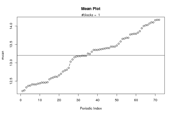
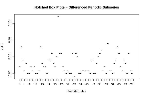
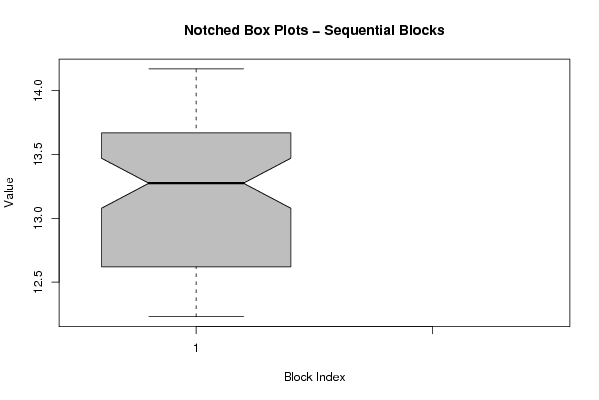
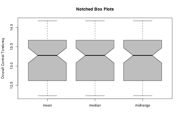
| Title produced by software | Mean Plot | ||||||||||||||||||||
| Date of computation | Mon, 28 Apr 2008 10:50:27 -0600 | ||||||||||||||||||||
| Cite this page as follows | Statistical Computations at FreeStatistics.org, Office for Research Development and Education, URL https://freestatistics.org/blog/index.php?v=date/2008/Apr/28/t1209401470adr3g114qhklffl.htm/, Retrieved Thu, 16 May 2024 13:54:45 +0000 | ||||||||||||||||||||
| Statistical Computations at FreeStatistics.org, Office for Research Development and Education, URL https://freestatistics.org/blog/index.php?pk=10944, Retrieved Thu, 16 May 2024 13:54:45 +0000 | |||||||||||||||||||||
| QR Codes: | |||||||||||||||||||||
|
| |||||||||||||||||||||
| Original text written by user: | |||||||||||||||||||||
| IsPrivate? | No (this computation is public) | ||||||||||||||||||||
| User-defined keywords | |||||||||||||||||||||
| Estimated Impact | 201 | ||||||||||||||||||||
Tree of Dependent Computations | |||||||||||||||||||||
| Family? (F = Feedback message, R = changed R code, M = changed R Module, P = changed Parameters, D = changed Data) | |||||||||||||||||||||
| - [Mean Plot] [] [2008-04-28 16:50:27] [0344071b671470f3024f96efc0c7614f] [Current] | |||||||||||||||||||||
| Feedback Forum | |||||||||||||||||||||
Post a new message | |||||||||||||||||||||
Dataset | |||||||||||||||||||||
| Dataseries X: | |||||||||||||||||||||
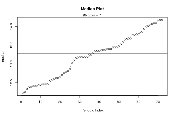
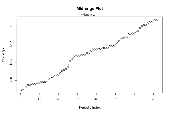
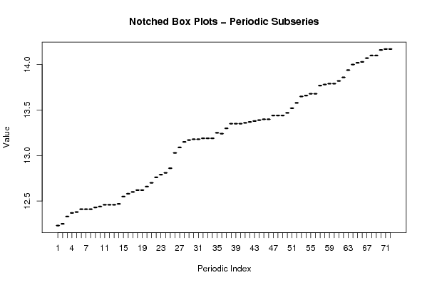
12,23 12,25 12,33 12,37 12,38 12,41 12,41 12,41 12,43 12,44 12,46 12,46 12,46 12,47 12,55 12,58 12,6 12,62 12,62 12,66 12,7 12,76 12,79 12,81 12,86 13,03 13,09 13,15 13,17 13,18 13,18 13,19 13,19 13,19 13,25 13,24 13,3 13,35 13,35 13,35 13,36 13,37 13,38 13,39 13,4 13,4 13,44 13,44 13,44 13,47 13,52 13,58 13,65 13,66 13,68 13,68 13,77 13,78 13,79 13,79 13,82 13,86 13,94 14 14,02 14,03 14,07 14,1 14,1 14,16 14,17 14,17 | |||||||||||||||||||||
Tables (Output of Computation) | |||||||||||||||||||||
| |||||||||||||||||||||
Figures (Output of Computation) | |||||||||||||||||||||
Input Parameters & R Code | |||||||||||||||||||||
| Parameters (Session): | |||||||||||||||||||||
| par1 = 72 ; | |||||||||||||||||||||
| Parameters (R input): | |||||||||||||||||||||
| par1 = 72 ; | |||||||||||||||||||||
| R code (references can be found in the software module): | |||||||||||||||||||||
par1 <- as.numeric(par1) | |||||||||||||||||||||