Free Statistics
of Irreproducible Research!
Description of Statistical Computation | |||||||||||||||||||||||||||||||||
|---|---|---|---|---|---|---|---|---|---|---|---|---|---|---|---|---|---|---|---|---|---|---|---|---|---|---|---|---|---|---|---|---|---|
| Author's title | |||||||||||||||||||||||||||||||||
| Author | *Unverified author* | ||||||||||||||||||||||||||||||||
| R Software Module | rwasp_meanversusmedian.wasp | ||||||||||||||||||||||||||||||||
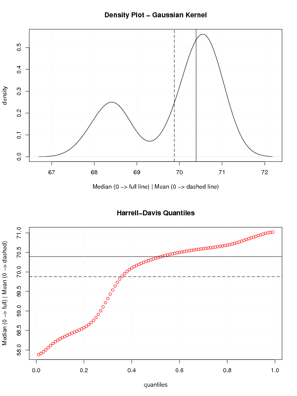
| Title produced by software | Mean versus Median | ||||||||||||||||||||||||||||||||
| Date of computation | Mon, 21 Apr 2008 14:41:06 -0600 | ||||||||||||||||||||||||||||||||
| Cite this page as follows | Statistical Computations at FreeStatistics.org, Office for Research Development and Education, URL https://freestatistics.org/blog/index.php?v=date/2008/Apr/21/t1208810621wb0col5balspjch.htm/, Retrieved Thu, 16 May 2024 22:47:18 +0000 | ||||||||||||||||||||||||||||||||
| Statistical Computations at FreeStatistics.org, Office for Research Development and Education, URL https://freestatistics.org/blog/index.php?pk=10605, Retrieved Thu, 16 May 2024 22:47:18 +0000 | |||||||||||||||||||||||||||||||||
| QR Codes: | |||||||||||||||||||||||||||||||||
|
| |||||||||||||||||||||||||||||||||
| Original text written by user: | |||||||||||||||||||||||||||||||||
| IsPrivate? | No (this computation is public) | ||||||||||||||||||||||||||||||||
| User-defined keywords | Eigen cijferreeks - vergelijking rek. gem. en mediaan | ||||||||||||||||||||||||||||||||
| Estimated Impact | 175 | ||||||||||||||||||||||||||||||||
Tree of Dependent Computations | |||||||||||||||||||||||||||||||||
| Family? (F = Feedback message, R = changed R code, M = changed R Module, P = changed Parameters, D = changed Data) | |||||||||||||||||||||||||||||||||
| - [] [Stephanie De Coni...] [-0001-11-30 00:00:00] [cd00afdb012dd785c94e77d4cae74ef4] - RM D [Mean versus Median] [Stephanie De Coni...] [2008-04-21 20:41:06] [80d88a38ebee1e39f846defee1b12cef] [Current] | |||||||||||||||||||||||||||||||||
| Feedback Forum | |||||||||||||||||||||||||||||||||
Post a new message | |||||||||||||||||||||||||||||||||
Dataset | |||||||||||||||||||||||||||||||||
| Dataseries X: | |||||||||||||||||||||||||||||||||
68.64 68.61 68.61 68.61 68.58 68.75 68.54 68.5 68.47 68.47 68.47 68.59 68.32 67.86 67.91 67.91 68.05 68.15 68.25 68.25 68.31 68.31 69.65 69.65 70.18 70.08 70.08 70.09 70.04 70.14 70.26 70.23 70.54 70.54 70.57 70.61 70.63 70.45 70.4 70.4 70.33 70.51 70.45 70.39 70.59 70.59 70.32 70.94 70.44 70.57 70.61 70.61 70.68 69.96 70.11 70.22 70.49 70.49 70.58 70.85 70.69 70.7 70.7 70.7 70.67 70.64 70.98 70.75 70.88 70.88 70.92 70.89 71.02 71.01 71.02 | |||||||||||||||||||||||||||||||||
Tables (Output of Computation) | |||||||||||||||||||||||||||||||||
| |||||||||||||||||||||||||||||||||
Figures (Output of Computation) | |||||||||||||||||||||||||||||||||
Input Parameters & R Code | |||||||||||||||||||||||||||||||||
| Parameters (Session): | |||||||||||||||||||||||||||||||||
| Parameters (R input): | |||||||||||||||||||||||||||||||||
| R code (references can be found in the software module): | |||||||||||||||||||||||||||||||||
library(Hmisc) | |||||||||||||||||||||||||||||||||