Free Statistics
of Irreproducible Research!
Description of Statistical Computation | |||||||||||||||||||||||||||||||||||||||||||||||||||||
|---|---|---|---|---|---|---|---|---|---|---|---|---|---|---|---|---|---|---|---|---|---|---|---|---|---|---|---|---|---|---|---|---|---|---|---|---|---|---|---|---|---|---|---|---|---|---|---|---|---|---|---|---|---|
| Author's title | |||||||||||||||||||||||||||||||||||||||||||||||||||||
| Author | *Unverified author* | ||||||||||||||||||||||||||||||||||||||||||||||||||||
| R Software Module | rwasp_edauni.wasp | ||||||||||||||||||||||||||||||||||||||||||||||||||||
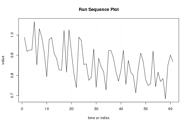
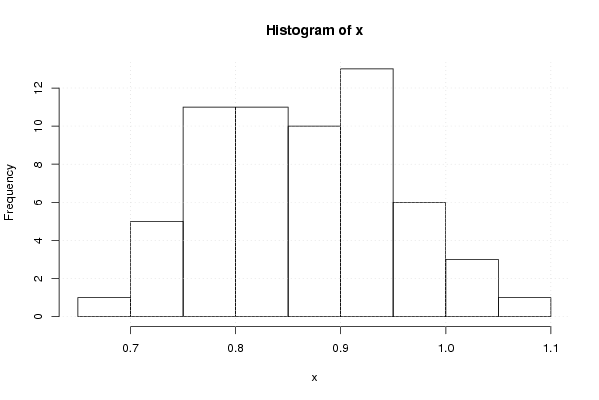
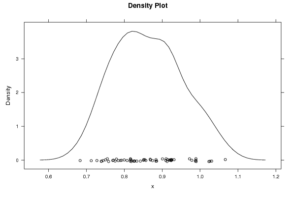
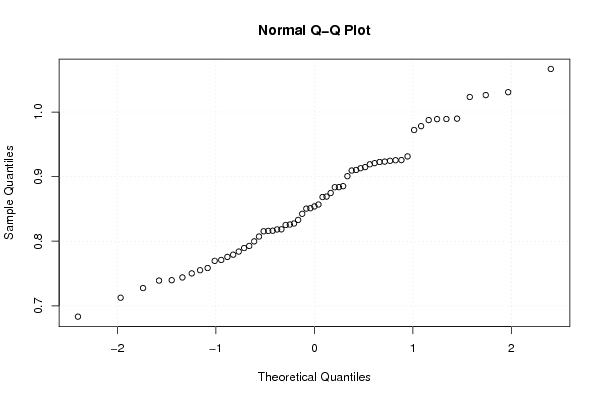
| Title produced by software | Univariate Explorative Data Analysis | ||||||||||||||||||||||||||||||||||||||||||||||||||||
| Date of computation | Sun, 21 Oct 2007 11:26:46 -0700 | ||||||||||||||||||||||||||||||||||||||||||||||||||||
| Cite this page as follows | Statistical Computations at FreeStatistics.org, Office for Research Development and Education, URL https://freestatistics.org/blog/index.php?v=date/2007/Oct/21/qyhnfd7xv3ynnau1192991194.htm/, Retrieved Thu, 09 May 2024 07:21:26 +0000 | ||||||||||||||||||||||||||||||||||||||||||||||||||||
| Statistical Computations at FreeStatistics.org, Office for Research Development and Education, URL https://freestatistics.org/blog/index.php?pk=1289, Retrieved Thu, 09 May 2024 07:21:26 +0000 | |||||||||||||||||||||||||||||||||||||||||||||||||||||
| QR Codes: | |||||||||||||||||||||||||||||||||||||||||||||||||||||
|
| |||||||||||||||||||||||||||||||||||||||||||||||||||||
| Original text written by user: | |||||||||||||||||||||||||||||||||||||||||||||||||||||
| IsPrivate? | No (this computation is public) | ||||||||||||||||||||||||||||||||||||||||||||||||||||
| User-defined keywords | Q3 Univariate explorative data analysis | ||||||||||||||||||||||||||||||||||||||||||||||||||||
| Estimated Impact | 479 | ||||||||||||||||||||||||||||||||||||||||||||||||||||
Tree of Dependent Computations | |||||||||||||||||||||||||||||||||||||||||||||||||||||
| Family? (F = Feedback message, R = changed R code, M = changed R Module, P = changed Parameters, D = changed Data) | |||||||||||||||||||||||||||||||||||||||||||||||||||||
| F [Univariate Explorative Data Analysis] [Investigating Dis...] [2007-10-21 18:26:46] [3cbd35878d9bd3c68c81c01c5c6ec146] [Current] F D [Univariate Explorative Data Analysis] [q3 univariate exp...] [2008-10-22 13:40:40] [7173087adebe3e3a714c80ea2417b3eb] F [Univariate Explorative Data Analysis] [q3] [2008-10-27 10:30:59] [e43247bc0ab243a5af99ac7f55ba0b41] F [Univariate Explorative Data Analysis] [Q3 Univariate Exp...] [2008-10-27 19:44:51] [c993f605b206b366f754f7f8c1fcc291] - R D [Univariate Explorative Data Analysis] [q3 Univariate exp...] [2008-10-22 13:57:47] [e43247bc0ab243a5af99ac7f55ba0b41] F R PD [Univariate Explorative Data Analysis] [Univariate EDA Q7...] [2008-10-22 14:37:05] [819b576fab25b35cfda70f80599828ec] - P [Univariate Explorative Data Analysis] [Q7 Univariate exp...] [2008-11-02 14:15:44] [d134696a922d84037f02d49ded84b0bd] - RMP [Central Tendency] [] [2008-11-03 08:48:28] [f5709eefd05c649ca6dad46019ffd879] F PD [Univariate Explorative Data Analysis] [Q3:] [2008-10-23 10:25:21] [cb714085b233acee8e8acd879ea442b6] - D [Univariate Explorative Data Analysis] [Univariate explor...] [2008-10-23 10:38:46] [adb6b6905cde49db36d59ca44433140d] F D [Univariate Explorative Data Analysis] [] [2008-10-23 10:41:45] [2a30350413961f11db13c46be07a5f73] - D [Univariate Explorative Data Analysis] [Q3:Univariate EDA] [2008-10-23 11:24:01] [1ce0d16c8f4225c977b42c8fa93bc163] - D [Univariate Explorative Data Analysis] [vraag 1: Q3 Growt...] [2008-10-23 11:28:10] [82d201ca7b4e7cd2c6f885d29b5b6937] F PD [Univariate Explorative Data Analysis] [Q3 met lags] [2008-10-23 13:08:11] [46c5a5fbda57fdfa1d4ef48658f82a0c] - [Univariate Explorative Data Analysis] [Q3] [2008-10-27 09:28:09] [b5373f20234c18c6452d5f98d8abf0fe] - RMP [Central Tendency] [Q3 verbetering] [2008-10-28 19:05:04] [46c5a5fbda57fdfa1d4ef48658f82a0c] - RMP [Central Tendency] [Q3 verbetering (2)] [2008-10-28 19:06:46] [46c5a5fbda57fdfa1d4ef48658f82a0c] - D [Univariate Explorative Data Analysis] [Q2 Investigating ...] [2008-10-23 13:14:55] [74be16979710d4c4e7c6647856088456] F D [Univariate Explorative Data Analysis] [Q3: Prove that gr...] [2008-10-23 13:30:10] [1e1d8320a8a1170c475bf6e4ce119de6] - [Univariate Explorative Data Analysis] [Q3: Prove that gr...] [2008-10-27 19:05:42] [988ab43f527fc78aae41c84649095267] - P [Univariate Explorative Data Analysis] [Seizoenailteit] [2008-11-03 21:03:22] [85841a4a203c2f9589565c024425a91b] - RMPD [Maximum-likelihood Fitting - Lognormal Distribution] [QQ Log] [2008-10-23 14:53:17] [46c5a5fbda57fdfa1d4ef48658f82a0c] - RMPD [Maximum-likelihood Fitting - Weibull Distribution] [QQ Weibull] [2008-10-23 14:54:45] [46c5a5fbda57fdfa1d4ef48658f82a0c] - RM [Maximum-likelihood Fitting - Gamma Distribution] [QQ Gamma] [2008-10-23 14:57:54] [46c5a5fbda57fdfa1d4ef48658f82a0c] - RMPD [Harrell-Davis Quantiles] [Q5 - distributions] [2008-10-23 16:14:37] [e5d91604aae608e98a8ea24759233f66] F D [Univariate Explorative Data Analysis] [Univariate explor...] [2008-10-23 18:32:20] [45822fdf1b746b5c6b4ce78e65a55a58] - [Univariate Explorative Data Analysis] [Investigation val...] [2008-10-27 21:42:21] [74be16979710d4c4e7c6647856088456] F D [Univariate Explorative Data Analysis] [Vraag 3] [2008-10-24 08:27:19] [87cabf13a90315c7085b765dcebb7412] F [Univariate Explorative Data Analysis] [Q3] [2008-10-27 21:38:01] [d2d412c7f4d35ffbf5ee5ee89db327d4] F D [Univariate Explorative Data Analysis] [Investigating dis...] [2008-10-24 08:58:00] [58bf45a666dc5198906262e8815a9722] - D [Univariate Explorative Data Analysis] [Q3 Clothing Produ...] [2008-10-24 09:47:35] [f9b9e85820b2a54b20380c3265aca831] F D [Univariate Explorative Data Analysis] [Prove that growth...] [2008-10-24 13:49:02] [1376d48f59a7212e8dd85a587491a69b] - D [Univariate Explorative Data Analysis] [Q3 Univariate Exp...] [2008-10-24 14:04:29] [7d3039e6253bb5fb3b26df1537d500b4] F D [Univariate Explorative Data Analysis] [Investigating Dis...] [2008-10-24 14:43:18] [063e4b67ad7d3a8a83eccec794cd5aa7] F [Univariate Explorative Data Analysis] [Investigating Dis...] [2008-10-24 15:00:51] [063e4b67ad7d3a8a83eccec794cd5aa7] F D [Univariate Explorative Data Analysis] [q3 inv distr] [2008-10-24 16:14:09] [8545382734d98368249ce527c6558129] F PD [Univariate Explorative Data Analysis] [herberekening vra...] [2008-10-24 15:58:05] [c45c87b96bbf32ffc2144fc37d767b2e] F D [Univariate Explorative Data Analysis] [Investigating Dis...] [2008-10-24 17:04:13] [a57f5cc542637534b8bb5bcb4d37eab1] F D [Univariate Explorative Data Analysis] [Investigating dis...] [2008-10-25 11:24:17] [2d4aec5ed1856c4828162be37be304d9] F D [Univariate Explorative Data Analysis] [Investigating dis...] [2008-10-27 18:03:14] [2d4aec5ed1856c4828162be37be304d9] F D [Univariate Explorative Data Analysis] [Investigating Dis...] [2008-10-25 12:18:54] [6743688719638b0cb1c0a6e0bf433315] F D [Univariate Explorative Data Analysis] [Q3] [2008-10-25 12:44:46] [b187fac1a1b0cb3920f54366df47fea3] - D [Univariate Explorative Data Analysis] [Q3 U EDA] [2008-10-25 16:56:45] [547636b63517c1c2916a747d66b36ebf] F D [Univariate Explorative Data Analysis] [Investigating Dis...] [2008-10-25 20:12:43] [b82ef11dce0545f3fd4676ec3ebed828] - D [Univariate Explorative Data Analysis] [Investigating dis...] [2008-10-25 20:28:11] [d32f94eec6fe2d8c421bd223368a5ced] - [Univariate Explorative Data Analysis] [] [2008-11-03 13:50:00] [888addc516c3b812dd7be4bd54caa358] - [Univariate Explorative Data Analysis] [] [2008-11-03 13:52:34] [888addc516c3b812dd7be4bd54caa358] - [Univariate Explorative Data Analysis] [] [2008-11-03 14:01:41] [888addc516c3b812dd7be4bd54caa358] - [Univariate Explorative Data Analysis] [] [2008-11-03 14:59:06] [888addc516c3b812dd7be4bd54caa358] [Truncated] | |||||||||||||||||||||||||||||||||||||||||||||||||||||
| Feedback Forum | |||||||||||||||||||||||||||||||||||||||||||||||||||||
Post a new message | |||||||||||||||||||||||||||||||||||||||||||||||||||||
Dataset | |||||||||||||||||||||||||||||||||||||||||||||||||||||
| Dataseries X: | |||||||||||||||||||||||||||||||||||||||||||||||||||||
0.989130435 0.919087137 0.925417076 0.925612053 1.066666667 0.851108765 1.030693069 0.989031079 0.913000978 0.792723264 0.978170478 0.987513007 0.909433962 0.883608147 0.82745098 0.8252149 1.023255814 0.815418024 1.026192703 0.914742451 0.807276303 0.739130435 0.98973306 0.972164948 0.853889943 0.856864654 0.775739042 0.789473684 0.931350114 0.73971079 0.885245902 0.842435094 0.818458418 0.72755418 0.923238696 0.922680412 0.883762201 0.818270165 0.771047228 0.825852783 0.924485126 0.755165289 0.874671341 0.815956482 0.799807507 0.712598425 0.832980973 0.910323253 0.869149952 0.779182879 0.750254842 0.75856014 0.920889988 0.743991641 0.816254417 0.769593957 0.784007353 0.683284457 0.850505051 0.900695134 0.868398268 | |||||||||||||||||||||||||||||||||||||||||||||||||||||
Tables (Output of Computation) | |||||||||||||||||||||||||||||||||||||||||||||||||||||
| |||||||||||||||||||||||||||||||||||||||||||||||||||||
Figures (Output of Computation) | |||||||||||||||||||||||||||||||||||||||||||||||||||||
Input Parameters & R Code | |||||||||||||||||||||||||||||||||||||||||||||||||||||
| Parameters (Session): | |||||||||||||||||||||||||||||||||||||||||||||||||||||
| par1 = 0 ; par2 = 0 ; | |||||||||||||||||||||||||||||||||||||||||||||||||||||
| Parameters (R input): | |||||||||||||||||||||||||||||||||||||||||||||||||||||
| par1 = 0 ; par2 = 0 ; | |||||||||||||||||||||||||||||||||||||||||||||||||||||
| R code (references can be found in the software module): | |||||||||||||||||||||||||||||||||||||||||||||||||||||
par1 <- as.numeric(par1) | |||||||||||||||||||||||||||||||||||||||||||||||||||||