Repository of Reproducible Computations

Free Statistics

of Irreproducible Research!

Author's title

Author

*Unverified author*

R Software Module

rwasp_autocorrelation.wasp

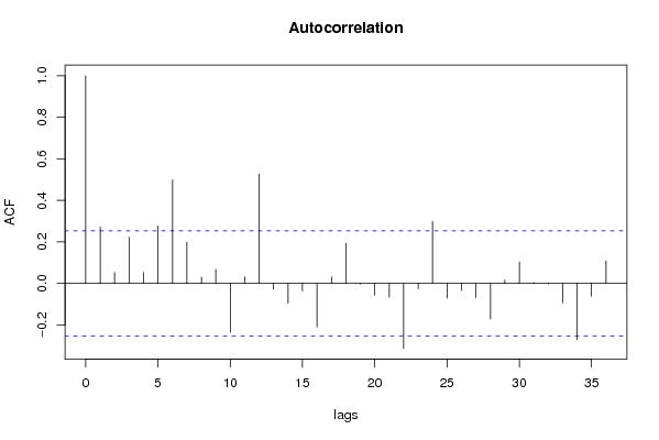
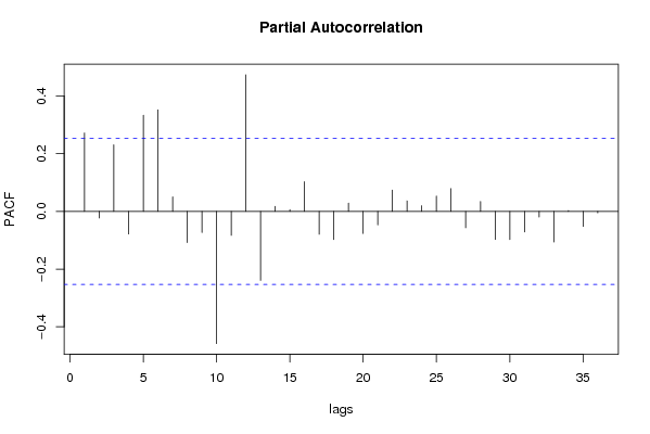
Title produced by software

(Partial) Autocorrelation Function

Date of computation

Sat, 01 Dec 2007 05:01:15 -0700

Cite this page as follows

Statistical Computations at FreeStatistics.org, Office for Research Development and Education, URL https://freestatistics.org/blog/index.php?v=date/2007/Dec/01/t1196509845zaas9urr338b49h.htm/, Retrieved Sun, 19 May 2024 19:55:57 +0000

Statistical Computations at FreeStatistics.org, Office for Research Development and Education, URL https://freestatistics.org/blog/index.php?pk=2219, Retrieved Sun, 19 May 2024 19:55:57 +0000

QR Codes:

Paste this QR Code to cite your computation.

Original text written by user:

IsPrivate?

No (this computation is public)

User-defined keywords

Estimated Impact

264

Family? (F = Feedback message, R = changed R code, M = changed R Module, P = changed Parameters, D = changed Data)

-       [(Partial) Autocorrelation Function] [paper auto 1] [2007-12-01 12:01:15] [fef19078983b9fa83d10cb717d6f9786] [Current]
-    D    [(Partial) Autocorrelation Function] [autocorrelation m...] [2008-12-16 19:08:07] [4ddbf81f78ea7c738951638c7e93f6ee] 
-    D      [(Partial) Autocorrelation Function] [autocorrelation v...] [2008-12-16 19:09:49] [4ddbf81f78ea7c738951638c7e93f6ee] 
-    D        [(Partial) Autocorrelation Function] [autocorrelation t...] [2008-12-16 19:11:22] [4ddbf81f78ea7c738951638c7e93f6ee] 
-   PD          [(Partial) Autocorrelation Function] [autocorrelation d...] [2008-12-18 13:47:38] [4ddbf81f78ea7c738951638c7e93f6ee] 
-   P             [(Partial) Autocorrelation Function] [autocorrelation d...] [2008-12-18 13:55:00] [4ddbf81f78ea7c738951638c7e93f6ee] 
-   PD        [(Partial) Autocorrelation Function] [autocorrelation d...] [2008-12-18 13:34:54] [4ddbf81f78ea7c738951638c7e93f6ee] 
-   P           [(Partial) Autocorrelation Function] [autocorrelation d...] [2008-12-18 13:39:29] [4ddbf81f78ea7c738951638c7e93f6ee] 
-   P             [(Partial) Autocorrelation Function] [autocorrelation d...] [2008-12-18 13:42:39] [4ddbf81f78ea7c738951638c7e93f6ee] 
-   PD      [(Partial) Autocorrelation Function] [autocorrelation d...] [2008-12-18 13:22:45] [4ddbf81f78ea7c738951638c7e93f6ee] 
- R PD    [(Partial) Autocorrelation Function] [Paper - autocorre...] [2008-12-21 15:54:30] [1848c1c05ef454c234bcbe26cf08badc] 
-   P       [(Partial) Autocorrelation Function] [Paper - ACF lambd...] [2008-12-22 12:33:54] [1848c1c05ef454c234bcbe26cf08badc] 
- R PD    [(Partial) Autocorrelation Function] [Autocorrelation e...] [2008-12-22 07:48:52] [74be16979710d4c4e7c6647856088456] 
- RMPD    [Spectral Analysis] [Paper - cumulativ...] [2008-12-22 08:58:23] [1848c1c05ef454c234bcbe26cf08badc] 
- RMPD    [Spectral Analysis] [Paper - cumulativ...] [2008-12-22 09:18:18] [1848c1c05ef454c234bcbe26cf08badc] 

Feedback Forum

Post a new message

Dataseries X:

Download CSV

Histogram

Boxplots

Summary of compuational transaction
Raw Input	view raw input (R code)
Raw Output	view raw output of R engine
Computing time	1 seconds
R Server	'Gwilym Jenkins' @ 72.249.127.135

\begin{tabular}{lllllllll}
\hline
Summary of compuational transaction \tabularnewline
Raw Input & view raw input (R code)  \tabularnewline
Raw Output & view raw output of R engine  \tabularnewline
Computing time & 1 seconds \tabularnewline
R Server & 'Gwilym Jenkins' @ 72.249.127.135 \tabularnewline
\hline
\end{tabular}
%Source: https://freestatistics.org/blog/index.php?pk=2219&T=0

[TABLE]
[ROW][C]Summary of compuational transaction[/C][/ROW]
[ROW][C]Raw Input[/C][C]view raw input (R code) [/C][/ROW]
[ROW][C]Raw Output[/C][C]view raw output of R engine [/C][/ROW]
[ROW][C]Computing time[/C][C]1 seconds[/C][/ROW]
[ROW][C]R Server[/C][C]'Gwilym Jenkins' @ 72.249.127.135[/C][/ROW]
[/TABLE]
Source: https://freestatistics.org/blog/index.php?pk=2219&T=0

Globally Unique Identifier (entire table): ba.freestatistics.org/blog/index.php?pk=2219&T=0

As an alternative you can also use a QR Code:

The GUIDs for individual cells are displayed in the table below:

Summary of compuational transaction
Raw Input	view raw input (R code)
Raw Output	view raw output of R engine
Computing time	1 seconds
R Server	'Gwilym Jenkins' @ 72.249.127.135

Autocorrelation Function
Time lag k	ACF(k)	T-STAT	P-value
0	1	7.746	0
1	0.271776	2.1052	0.019736
2	0.052583	0.4073	0.342617
3	0.221954	1.7192	0.045362
4	0.05211	0.4036	0.343956
5	0.277076	2.1462	0.017955
6	0.498494	3.8613	0.000139
7	0.197897	1.5329	0.065278
8	0.029509	0.2286	0.409987
9	0.067472	0.5226	0.301576
10	-0.235237	-1.8221	0.963291
11	0.03201	0.248	0.402509
12	0.527214	4.0838	6.7e-05
13	-0.028279	-0.2191	0.586323
14	-0.096099	-0.7444	0.770223
15	-0.036252	-0.2808	0.610087
16	-0.209634	-1.6238	0.945171
17	0.031279	0.2423	0.404692
18	0.192956	1.4946	0.070126
19	-0.003704	-0.0287	0.511396
20	-0.057958	-0.4489	0.672455
21	-0.067029	-0.5192	0.697235
22	-0.312668	-2.4219	0.990761
23	-0.025235	-0.1955	0.577156
24	0.299579	2.3205	0.011865
25	-0.071215	-0.5516	0.708373
26	-0.033885	-0.2625	0.603071
27	-0.067877	-0.5258	0.699507
28	-0.171925	-1.3317	0.906006
29	0.017142	0.1328	0.447405
30	0.103593	0.8024	0.212736
31	0.004165	0.0323	0.487184
32	-0.002063	-0.016	0.506347
33	-0.093224	-0.7221	0.763484
34	-0.271677	-2.1044	0.980229
35	-0.062024	-0.4804	0.683667

\begin{tabular}{lllllllll}
\hline
Autocorrelation Function \tabularnewline
Time lag k & ACF(k) & T-STAT & P-value \tabularnewline
0 & 1 & 7.746 & 0 \tabularnewline
1 & 0.271776 & 2.1052 & 0.019736 \tabularnewline
2 & 0.052583 & 0.4073 & 0.342617 \tabularnewline
3 & 0.221954 & 1.7192 & 0.045362 \tabularnewline
4 & 0.05211 & 0.4036 & 0.343956 \tabularnewline
5 & 0.277076 & 2.1462 & 0.017955 \tabularnewline
6 & 0.498494 & 3.8613 & 0.000139 \tabularnewline
7 & 0.197897 & 1.5329 & 0.065278 \tabularnewline
8 & 0.029509 & 0.2286 & 0.409987 \tabularnewline
9 & 0.067472 & 0.5226 & 0.301576 \tabularnewline
10 & -0.235237 & -1.8221 & 0.963291 \tabularnewline
11 & 0.03201 & 0.248 & 0.402509 \tabularnewline
12 & 0.527214 & 4.0838 & 6.7e-05 \tabularnewline
13 & -0.028279 & -0.2191 & 0.586323 \tabularnewline
14 & -0.096099 & -0.7444 & 0.770223 \tabularnewline
15 & -0.036252 & -0.2808 & 0.610087 \tabularnewline
16 & -0.209634 & -1.6238 & 0.945171 \tabularnewline
17 & 0.031279 & 0.2423 & 0.404692 \tabularnewline
18 & 0.192956 & 1.4946 & 0.070126 \tabularnewline
19 & -0.003704 & -0.0287 & 0.511396 \tabularnewline
20 & -0.057958 & -0.4489 & 0.672455 \tabularnewline
21 & -0.067029 & -0.5192 & 0.697235 \tabularnewline
22 & -0.312668 & -2.4219 & 0.990761 \tabularnewline
23 & -0.025235 & -0.1955 & 0.577156 \tabularnewline
24 & 0.299579 & 2.3205 & 0.011865 \tabularnewline
25 & -0.071215 & -0.5516 & 0.708373 \tabularnewline
26 & -0.033885 & -0.2625 & 0.603071 \tabularnewline
27 & -0.067877 & -0.5258 & 0.699507 \tabularnewline
28 & -0.171925 & -1.3317 & 0.906006 \tabularnewline
29 & 0.017142 & 0.1328 & 0.447405 \tabularnewline
30 & 0.103593 & 0.8024 & 0.212736 \tabularnewline
31 & 0.004165 & 0.0323 & 0.487184 \tabularnewline
32 & -0.002063 & -0.016 & 0.506347 \tabularnewline
33 & -0.093224 & -0.7221 & 0.763484 \tabularnewline
34 & -0.271677 & -2.1044 & 0.980229 \tabularnewline
35 & -0.062024 & -0.4804 & 0.683667 \tabularnewline
\hline
\end{tabular}
%Source: https://freestatistics.org/blog/index.php?pk=2219&T=1

[TABLE]
[ROW][C]Autocorrelation Function[/C][/ROW]
[ROW][C]Time lag k[/C][C]ACF(k)[/C][C]T-STAT[/C][C]P-value[/C][/ROW]
[ROW][C]0[/C][C]1[/C][C]7.746[/C][C]0[/C][/ROW]
[ROW][C]1[/C][C]0.271776[/C][C]2.1052[/C][C]0.019736[/C][/ROW]
[ROW][C]2[/C][C]0.052583[/C][C]0.4073[/C][C]0.342617[/C][/ROW]
[ROW][C]3[/C][C]0.221954[/C][C]1.7192[/C][C]0.045362[/C][/ROW]
[ROW][C]4[/C][C]0.05211[/C][C]0.4036[/C][C]0.343956[/C][/ROW]
[ROW][C]5[/C][C]0.277076[/C][C]2.1462[/C][C]0.017955[/C][/ROW]
[ROW][C]6[/C][C]0.498494[/C][C]3.8613[/C][C]0.000139[/C][/ROW]
[ROW][C]7[/C][C]0.197897[/C][C]1.5329[/C][C]0.065278[/C][/ROW]
[ROW][C]8[/C][C]0.029509[/C][C]0.2286[/C][C]0.409987[/C][/ROW]
[ROW][C]9[/C][C]0.067472[/C][C]0.5226[/C][C]0.301576[/C][/ROW]
[ROW][C]10[/C][C]-0.235237[/C][C]-1.8221[/C][C]0.963291[/C][/ROW]
[ROW][C]11[/C][C]0.03201[/C][C]0.248[/C][C]0.402509[/C][/ROW]
[ROW][C]12[/C][C]0.527214[/C][C]4.0838[/C][C]6.7e-05[/C][/ROW]
[ROW][C]13[/C][C]-0.028279[/C][C]-0.2191[/C][C]0.586323[/C][/ROW]
[ROW][C]14[/C][C]-0.096099[/C][C]-0.7444[/C][C]0.770223[/C][/ROW]
[ROW][C]15[/C][C]-0.036252[/C][C]-0.2808[/C][C]0.610087[/C][/ROW]
[ROW][C]16[/C][C]-0.209634[/C][C]-1.6238[/C][C]0.945171[/C][/ROW]
[ROW][C]17[/C][C]0.031279[/C][C]0.2423[/C][C]0.404692[/C][/ROW]
[ROW][C]18[/C][C]0.192956[/C][C]1.4946[/C][C]0.070126[/C][/ROW]
[ROW][C]19[/C][C]-0.003704[/C][C]-0.0287[/C][C]0.511396[/C][/ROW]
[ROW][C]20[/C][C]-0.057958[/C][C]-0.4489[/C][C]0.672455[/C][/ROW]
[ROW][C]21[/C][C]-0.067029[/C][C]-0.5192[/C][C]0.697235[/C][/ROW]
[ROW][C]22[/C][C]-0.312668[/C][C]-2.4219[/C][C]0.990761[/C][/ROW]
[ROW][C]23[/C][C]-0.025235[/C][C]-0.1955[/C][C]0.577156[/C][/ROW]
[ROW][C]24[/C][C]0.299579[/C][C]2.3205[/C][C]0.011865[/C][/ROW]
[ROW][C]25[/C][C]-0.071215[/C][C]-0.5516[/C][C]0.708373[/C][/ROW]
[ROW][C]26[/C][C]-0.033885[/C][C]-0.2625[/C][C]0.603071[/C][/ROW]
[ROW][C]27[/C][C]-0.067877[/C][C]-0.5258[/C][C]0.699507[/C][/ROW]
[ROW][C]28[/C][C]-0.171925[/C][C]-1.3317[/C][C]0.906006[/C][/ROW]
[ROW][C]29[/C][C]0.017142[/C][C]0.1328[/C][C]0.447405[/C][/ROW]
[ROW][C]30[/C][C]0.103593[/C][C]0.8024[/C][C]0.212736[/C][/ROW]
[ROW][C]31[/C][C]0.004165[/C][C]0.0323[/C][C]0.487184[/C][/ROW]
[ROW][C]32[/C][C]-0.002063[/C][C]-0.016[/C][C]0.506347[/C][/ROW]
[ROW][C]33[/C][C]-0.093224[/C][C]-0.7221[/C][C]0.763484[/C][/ROW]
[ROW][C]34[/C][C]-0.271677[/C][C]-2.1044[/C][C]0.980229[/C][/ROW]
[ROW][C]35[/C][C]-0.062024[/C][C]-0.4804[/C][C]0.683667[/C][/ROW]
[/TABLE]
Source: https://freestatistics.org/blog/index.php?pk=2219&T=1

Globally Unique Identifier (entire table): ba.freestatistics.org/blog/index.php?pk=2219&T=1

As an alternative you can also use a QR Code:

The GUIDs for individual cells are displayed in the table below:

Autocorrelation Function
Time lag k	ACF(k)	T-STAT	P-value
0	1	7.746	0
1	0.271776	2.1052	0.019736
2	0.052583	0.4073	0.342617
3	0.221954	1.7192	0.045362
4	0.05211	0.4036	0.343956
5	0.277076	2.1462	0.017955
6	0.498494	3.8613	0.000139
7	0.197897	1.5329	0.065278
8	0.029509	0.2286	0.409987
9	0.067472	0.5226	0.301576
10	-0.235237	-1.8221	0.963291
11	0.03201	0.248	0.402509
12	0.527214	4.0838	6.7e-05
13	-0.028279	-0.2191	0.586323
14	-0.096099	-0.7444	0.770223
15	-0.036252	-0.2808	0.610087
16	-0.209634	-1.6238	0.945171
17	0.031279	0.2423	0.404692
18	0.192956	1.4946	0.070126
19	-0.003704	-0.0287	0.511396
20	-0.057958	-0.4489	0.672455
21	-0.067029	-0.5192	0.697235
22	-0.312668	-2.4219	0.990761
23	-0.025235	-0.1955	0.577156
24	0.299579	2.3205	0.011865
25	-0.071215	-0.5516	0.708373
26	-0.033885	-0.2625	0.603071
27	-0.067877	-0.5258	0.699507
28	-0.171925	-1.3317	0.906006
29	0.017142	0.1328	0.447405
30	0.103593	0.8024	0.212736
31	0.004165	0.0323	0.487184
32	-0.002063	-0.016	0.506347
33	-0.093224	-0.7221	0.763484
34	-0.271677	-2.1044	0.980229
35	-0.062024	-0.4804	0.683667

Partial Autocorrelation Function
Time lag k	PACF(k)	T-STAT	P-value
0	0.271776	2.1052	0.019736
1	-0.022977	-0.178	0.57033
2	0.230735	1.7873	0.039473
3	-0.078622	-0.609	0.727589
4	0.333301	2.5817	0.006145
5	0.352264	2.7286	0.004166
6	0.050179	0.3887	0.349442
7	-0.108026	-0.8368	0.796977
8	-0.073075	-0.566	0.713261
9	-0.458002	-3.5477	0.999619
10	-0.082927	-0.6424	0.738454
11	0.473267	3.6659	0.000262
12	-0.239164	-1.8526	0.965567
13	0.017414	0.1349	0.446577
14	0.00602	0.0466	0.481482
15	0.102773	0.7961	0.214564
16	-0.079379	-0.6149	0.729517
17	-0.097656	-0.7564	0.773828
18	0.028953	0.2243	0.411656
19	-0.076431	-0.592	0.721973
20	-0.046977	-0.3639	0.641387
21	0.073917	0.5726	0.284541
22	0.036491	0.2827	0.389205
23	0.019624	0.152	0.439847
24	0.053297	0.4128	0.3406
25	0.078918	0.6113	0.271658
26	-0.056865	-0.4405	0.669411
27	0.034337	0.266	0.395586
28	-0.097425	-0.7546	0.773294
29	-0.09779	-0.7575	0.774137
30	-0.071323	-0.5525	0.708659
31	-0.019659	-0.1523	0.560261
32	-0.106047	-0.8214	0.792674
33	0.002942	0.0228	0.490948
34	-0.052173	-0.4041	0.656224
35	-0.005121	-0.0397	0.515756

\begin{tabular}{lllllllll}
\hline
Partial Autocorrelation Function \tabularnewline
Time lag k & PACF(k) & T-STAT & P-value \tabularnewline
0 & 0.271776 & 2.1052 & 0.019736 \tabularnewline
1 & -0.022977 & -0.178 & 0.57033 \tabularnewline
2 & 0.230735 & 1.7873 & 0.039473 \tabularnewline
3 & -0.078622 & -0.609 & 0.727589 \tabularnewline
4 & 0.333301 & 2.5817 & 0.006145 \tabularnewline
5 & 0.352264 & 2.7286 & 0.004166 \tabularnewline
6 & 0.050179 & 0.3887 & 0.349442 \tabularnewline
7 & -0.108026 & -0.8368 & 0.796977 \tabularnewline
8 & -0.073075 & -0.566 & 0.713261 \tabularnewline
9 & -0.458002 & -3.5477 & 0.999619 \tabularnewline
10 & -0.082927 & -0.6424 & 0.738454 \tabularnewline
11 & 0.473267 & 3.6659 & 0.000262 \tabularnewline
12 & -0.239164 & -1.8526 & 0.965567 \tabularnewline
13 & 0.017414 & 0.1349 & 0.446577 \tabularnewline
14 & 0.00602 & 0.0466 & 0.481482 \tabularnewline
15 & 0.102773 & 0.7961 & 0.214564 \tabularnewline
16 & -0.079379 & -0.6149 & 0.729517 \tabularnewline
17 & -0.097656 & -0.7564 & 0.773828 \tabularnewline
18 & 0.028953 & 0.2243 & 0.411656 \tabularnewline
19 & -0.076431 & -0.592 & 0.721973 \tabularnewline
20 & -0.046977 & -0.3639 & 0.641387 \tabularnewline
21 & 0.073917 & 0.5726 & 0.284541 \tabularnewline
22 & 0.036491 & 0.2827 & 0.389205 \tabularnewline
23 & 0.019624 & 0.152 & 0.439847 \tabularnewline
24 & 0.053297 & 0.4128 & 0.3406 \tabularnewline
25 & 0.078918 & 0.6113 & 0.271658 \tabularnewline
26 & -0.056865 & -0.4405 & 0.669411 \tabularnewline
27 & 0.034337 & 0.266 & 0.395586 \tabularnewline
28 & -0.097425 & -0.7546 & 0.773294 \tabularnewline
29 & -0.09779 & -0.7575 & 0.774137 \tabularnewline
30 & -0.071323 & -0.5525 & 0.708659 \tabularnewline
31 & -0.019659 & -0.1523 & 0.560261 \tabularnewline
32 & -0.106047 & -0.8214 & 0.792674 \tabularnewline
33 & 0.002942 & 0.0228 & 0.490948 \tabularnewline
34 & -0.052173 & -0.4041 & 0.656224 \tabularnewline
35 & -0.005121 & -0.0397 & 0.515756 \tabularnewline
\hline
\end{tabular}
%Source: https://freestatistics.org/blog/index.php?pk=2219&T=2

[TABLE]
[ROW][C]Partial Autocorrelation Function[/C][/ROW]
[ROW][C]Time lag k[/C][C]PACF(k)[/C][C]T-STAT[/C][C]P-value[/C][/ROW]
[ROW][C]0[/C][C]0.271776[/C][C]2.1052[/C][C]0.019736[/C][/ROW]
[ROW][C]1[/C][C]-0.022977[/C][C]-0.178[/C][C]0.57033[/C][/ROW]
[ROW][C]2[/C][C]0.230735[/C][C]1.7873[/C][C]0.039473[/C][/ROW]
[ROW][C]3[/C][C]-0.078622[/C][C]-0.609[/C][C]0.727589[/C][/ROW]
[ROW][C]4[/C][C]0.333301[/C][C]2.5817[/C][C]0.006145[/C][/ROW]
[ROW][C]5[/C][C]0.352264[/C][C]2.7286[/C][C]0.004166[/C][/ROW]
[ROW][C]6[/C][C]0.050179[/C][C]0.3887[/C][C]0.349442[/C][/ROW]
[ROW][C]7[/C][C]-0.108026[/C][C]-0.8368[/C][C]0.796977[/C][/ROW]
[ROW][C]8[/C][C]-0.073075[/C][C]-0.566[/C][C]0.713261[/C][/ROW]
[ROW][C]9[/C][C]-0.458002[/C][C]-3.5477[/C][C]0.999619[/C][/ROW]
[ROW][C]10[/C][C]-0.082927[/C][C]-0.6424[/C][C]0.738454[/C][/ROW]
[ROW][C]11[/C][C]0.473267[/C][C]3.6659[/C][C]0.000262[/C][/ROW]
[ROW][C]12[/C][C]-0.239164[/C][C]-1.8526[/C][C]0.965567[/C][/ROW]
[ROW][C]13[/C][C]0.017414[/C][C]0.1349[/C][C]0.446577[/C][/ROW]
[ROW][C]14[/C][C]0.00602[/C][C]0.0466[/C][C]0.481482[/C][/ROW]
[ROW][C]15[/C][C]0.102773[/C][C]0.7961[/C][C]0.214564[/C][/ROW]
[ROW][C]16[/C][C]-0.079379[/C][C]-0.6149[/C][C]0.729517[/C][/ROW]
[ROW][C]17[/C][C]-0.097656[/C][C]-0.7564[/C][C]0.773828[/C][/ROW]
[ROW][C]18[/C][C]0.028953[/C][C]0.2243[/C][C]0.411656[/C][/ROW]
[ROW][C]19[/C][C]-0.076431[/C][C]-0.592[/C][C]0.721973[/C][/ROW]
[ROW][C]20[/C][C]-0.046977[/C][C]-0.3639[/C][C]0.641387[/C][/ROW]
[ROW][C]21[/C][C]0.073917[/C][C]0.5726[/C][C]0.284541[/C][/ROW]
[ROW][C]22[/C][C]0.036491[/C][C]0.2827[/C][C]0.389205[/C][/ROW]
[ROW][C]23[/C][C]0.019624[/C][C]0.152[/C][C]0.439847[/C][/ROW]
[ROW][C]24[/C][C]0.053297[/C][C]0.4128[/C][C]0.3406[/C][/ROW]
[ROW][C]25[/C][C]0.078918[/C][C]0.6113[/C][C]0.271658[/C][/ROW]
[ROW][C]26[/C][C]-0.056865[/C][C]-0.4405[/C][C]0.669411[/C][/ROW]
[ROW][C]27[/C][C]0.034337[/C][C]0.266[/C][C]0.395586[/C][/ROW]
[ROW][C]28[/C][C]-0.097425[/C][C]-0.7546[/C][C]0.773294[/C][/ROW]
[ROW][C]29[/C][C]-0.09779[/C][C]-0.7575[/C][C]0.774137[/C][/ROW]
[ROW][C]30[/C][C]-0.071323[/C][C]-0.5525[/C][C]0.708659[/C][/ROW]
[ROW][C]31[/C][C]-0.019659[/C][C]-0.1523[/C][C]0.560261[/C][/ROW]
[ROW][C]32[/C][C]-0.106047[/C][C]-0.8214[/C][C]0.792674[/C][/ROW]
[ROW][C]33[/C][C]0.002942[/C][C]0.0228[/C][C]0.490948[/C][/ROW]
[ROW][C]34[/C][C]-0.052173[/C][C]-0.4041[/C][C]0.656224[/C][/ROW]
[ROW][C]35[/C][C]-0.005121[/C][C]-0.0397[/C][C]0.515756[/C][/ROW]
[/TABLE]
Source: https://freestatistics.org/blog/index.php?pk=2219&T=2

Globally Unique Identifier (entire table): ba.freestatistics.org/blog/index.php?pk=2219&T=2

As an alternative you can also use a QR Code:

The GUIDs for individual cells are displayed in the table below:

Partial Autocorrelation Function
Time lag k	PACF(k)	T-STAT	P-value
0	0.271776	2.1052	0.019736
1	-0.022977	-0.178	0.57033
2	0.230735	1.7873	0.039473
3	-0.078622	-0.609	0.727589
4	0.333301	2.5817	0.006145
5	0.352264	2.7286	0.004166
6	0.050179	0.3887	0.349442
7	-0.108026	-0.8368	0.796977
8	-0.073075	-0.566	0.713261
9	-0.458002	-3.5477	0.999619
10	-0.082927	-0.6424	0.738454
11	0.473267	3.6659	0.000262
12	-0.239164	-1.8526	0.965567
13	0.017414	0.1349	0.446577
14	0.00602	0.0466	0.481482
15	0.102773	0.7961	0.214564
16	-0.079379	-0.6149	0.729517
17	-0.097656	-0.7564	0.773828
18	0.028953	0.2243	0.411656
19	-0.076431	-0.592	0.721973
20	-0.046977	-0.3639	0.641387
21	0.073917	0.5726	0.284541
22	0.036491	0.2827	0.389205
23	0.019624	0.152	0.439847
24	0.053297	0.4128	0.3406
25	0.078918	0.6113	0.271658
26	-0.056865	-0.4405	0.669411
27	0.034337	0.266	0.395586
28	-0.097425	-0.7546	0.773294
29	-0.09779	-0.7575	0.774137
30	-0.071323	-0.5525	0.708659
31	-0.019659	-0.1523	0.560261
32	-0.106047	-0.8214	0.792674
33	0.002942	0.0228	0.490948
34	-0.052173	-0.4041	0.656224
35	-0.005121	-0.0397	0.515756

Figure 1

PNG link

Postscript link

PDF link

Figure 2

PNG link

Postscript link

PDF link

Parameters (Session):

par1 = 36 ; par2 = 1 ; par3 = 0 ; par4 = 0 ; par5 = 12 ;

Parameters (R input):

par1 = 36 ; par2 = 1 ; par3 = 0 ; par4 = 0 ; par5 = 12 ;

R code (references can be found in the software module):

if (par1 == 'Default') {
par1 = 10*log10(length(x))
} else {
par1 <- as.numeric(par1)
}
par2 <- as.numeric(par2)
par3 <- as.numeric(par3)
par4 <- as.numeric(par4)
par5 <- as.numeric(par5)
if (par2 == 0) {
x <- log(x)
} else {
x <- (x ^ par2 - 1) / par2
}
if (par3 > 0) x <- diff(x,lag=1,difference=par3)
if (par4 > 0) x <- diff(x,lag=par5,difference=par4)
bitmap(file='pic1.png')
racf <- acf(x,par1,main='Autocorrelation',xlab='lags',ylab='ACF')
dev.off()
bitmap(file='pic2.png')
rpacf <- pacf(x,par1,main='Partial Autocorrelation',xlab='lags',ylab='PACF')
dev.off()
(myacf <- c(racf$acf))
(mypacf <- c(rpacf$acf))
lengthx <- length(x)
sqrtn <- sqrt(lengthx)
load(file='createtable')
a<-table.start()
a<-table.row.start(a)
a<-table.element(a,'Autocorrelation Function',4,TRUE)
a<-table.row.end(a)
a<-table.row.start(a)
a<-table.element(a,'Time lag k',header=TRUE)
a<-table.element(a,hyperlink('basics.htm','ACF(k)','click here for more information about the Autocorrelation Function'),header=TRUE)
a<-table.element(a,'T-STAT',header=TRUE)
a<-table.element(a,'P-value',header=TRUE)
a<-table.row.end(a)
for (i in 1:par1) {
a<-table.row.start(a)
a<-table.element(a,i-1,header=TRUE)
a<-table.element(a,round(myacf[i],6))
mytstat <- myacf[i]*sqrtn
a<-table.element(a,round(mytstat,4))
a<-table.element(a,round(1-pt(mytstat,lengthx),6))
a<-table.row.end(a)
}
a<-table.end(a)
table.save(a,file='mytable.tab')
a<-table.start()
a<-table.row.start(a)
a<-table.element(a,'Partial Autocorrelation Function',4,TRUE)
a<-table.row.end(a)
a<-table.row.start(a)
a<-table.element(a,'Time lag k',header=TRUE)
a<-table.element(a,hyperlink('basics.htm','PACF(k)','click here for more information about the Partial Autocorrelation Function'),header=TRUE)
a<-table.element(a,'T-STAT',header=TRUE)
a<-table.element(a,'P-value',header=TRUE)
a<-table.row.end(a)
for (i in 1:par1) {
a<-table.row.start(a)
a<-table.element(a,i-1,header=TRUE)
a<-table.element(a,round(mypacf[i],6))
mytstat <- mypacf[i]*sqrtn
a<-table.element(a,round(mytstat,4))
a<-table.element(a,round(1-pt(mytstat,lengthx),6))
a<-table.row.end(a)
}
a<-table.end(a)
table.save(a,file='mytable1.tab')

Free Statistics

Description of Statistical Computation

Tree of Dependent Computations

Dataset

Tables (Output of Computation)

Figures (Output of Computation)

Input Parameters & R Code