Free Statistics
of Irreproducible Research!
Description of Statistical Computation | |||||||||||||||||||||||||||||||||||||||||||||||||||||||||||||||||||||||||||||||||||||||||||||||||||||||||||||||||||||||||||||||||||||||||||||||||||||||||||||||||||||||||||||||||||||||||||||||||||||||||||||||||||||||||||||||||||||||||||||||||||||||||||||||||||||||||||
|---|---|---|---|---|---|---|---|---|---|---|---|---|---|---|---|---|---|---|---|---|---|---|---|---|---|---|---|---|---|---|---|---|---|---|---|---|---|---|---|---|---|---|---|---|---|---|---|---|---|---|---|---|---|---|---|---|---|---|---|---|---|---|---|---|---|---|---|---|---|---|---|---|---|---|---|---|---|---|---|---|---|---|---|---|---|---|---|---|---|---|---|---|---|---|---|---|---|---|---|---|---|---|---|---|---|---|---|---|---|---|---|---|---|---|---|---|---|---|---|---|---|---|---|---|---|---|---|---|---|---|---|---|---|---|---|---|---|---|---|---|---|---|---|---|---|---|---|---|---|---|---|---|---|---|---|---|---|---|---|---|---|---|---|---|---|---|---|---|---|---|---|---|---|---|---|---|---|---|---|---|---|---|---|---|---|---|---|---|---|---|---|---|---|---|---|---|---|---|---|---|---|---|---|---|---|---|---|---|---|---|---|---|---|---|---|---|---|---|---|---|---|---|---|---|---|---|---|---|---|---|---|---|---|---|---|---|---|---|---|---|---|---|---|---|---|---|---|---|---|---|---|---|---|---|---|---|---|---|---|---|---|---|---|---|---|---|---|
| Author's title | |||||||||||||||||||||||||||||||||||||||||||||||||||||||||||||||||||||||||||||||||||||||||||||||||||||||||||||||||||||||||||||||||||||||||||||||||||||||||||||||||||||||||||||||||||||||||||||||||||||||||||||||||||||||||||||||||||||||||||||||||||||||||||||||||||||||||||
| Author | *The author of this computation has been verified* | ||||||||||||||||||||||||||||||||||||||||||||||||||||||||||||||||||||||||||||||||||||||||||||||||||||||||||||||||||||||||||||||||||||||||||||||||||||||||||||||||||||||||||||||||||||||||||||||||||||||||||||||||||||||||||||||||||||||||||||||||||||||||||||||||||||||||||
| R Software Module | rwasp_Two Factor ANOVA.wasp | ||||||||||||||||||||||||||||||||||||||||||||||||||||||||||||||||||||||||||||||||||||||||||||||||||||||||||||||||||||||||||||||||||||||||||||||||||||||||||||||||||||||||||||||||||||||||||||||||||||||||||||||||||||||||||||||||||||||||||||||||||||||||||||||||||||||||||
| Title produced by software | Two-Way ANOVA | ||||||||||||||||||||||||||||||||||||||||||||||||||||||||||||||||||||||||||||||||||||||||||||||||||||||||||||||||||||||||||||||||||||||||||||||||||||||||||||||||||||||||||||||||||||||||||||||||||||||||||||||||||||||||||||||||||||||||||||||||||||||||||||||||||||||||||
| Date of computation | Mon, 28 Nov 2011 12:22:56 -0500 | ||||||||||||||||||||||||||||||||||||||||||||||||||||||||||||||||||||||||||||||||||||||||||||||||||||||||||||||||||||||||||||||||||||||||||||||||||||||||||||||||||||||||||||||||||||||||||||||||||||||||||||||||||||||||||||||||||||||||||||||||||||||||||||||||||||||||||
| Cite this page as follows | Statistical Computations at FreeStatistics.org, Office for Research Development and Education, URL https://freestatistics.org/blog/index.php?v=date/2011/Nov/28/t1322501153v09fnykfm4b4ef1.htm/, Retrieved Wed, 09 Jul 2025 12:37:39 +0000 | ||||||||||||||||||||||||||||||||||||||||||||||||||||||||||||||||||||||||||||||||||||||||||||||||||||||||||||||||||||||||||||||||||||||||||||||||||||||||||||||||||||||||||||||||||||||||||||||||||||||||||||||||||||||||||||||||||||||||||||||||||||||||||||||||||||||||||
| Statistical Computations at FreeStatistics.org, Office for Research Development and Education, URL https://freestatistics.org/blog/index.php?pk=147905, Retrieved Wed, 09 Jul 2025 12:37:39 +0000 | |||||||||||||||||||||||||||||||||||||||||||||||||||||||||||||||||||||||||||||||||||||||||||||||||||||||||||||||||||||||||||||||||||||||||||||||||||||||||||||||||||||||||||||||||||||||||||||||||||||||||||||||||||||||||||||||||||||||||||||||||||||||||||||||||||||||||||
| QR Codes: | |||||||||||||||||||||||||||||||||||||||||||||||||||||||||||||||||||||||||||||||||||||||||||||||||||||||||||||||||||||||||||||||||||||||||||||||||||||||||||||||||||||||||||||||||||||||||||||||||||||||||||||||||||||||||||||||||||||||||||||||||||||||||||||||||||||||||||
|
| |||||||||||||||||||||||||||||||||||||||||||||||||||||||||||||||||||||||||||||||||||||||||||||||||||||||||||||||||||||||||||||||||||||||||||||||||||||||||||||||||||||||||||||||||||||||||||||||||||||||||||||||||||||||||||||||||||||||||||||||||||||||||||||||||||||||||||
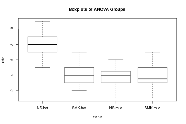
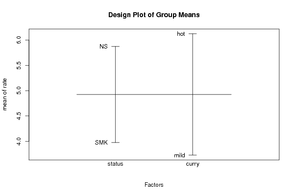
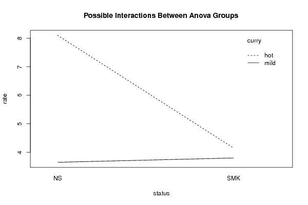
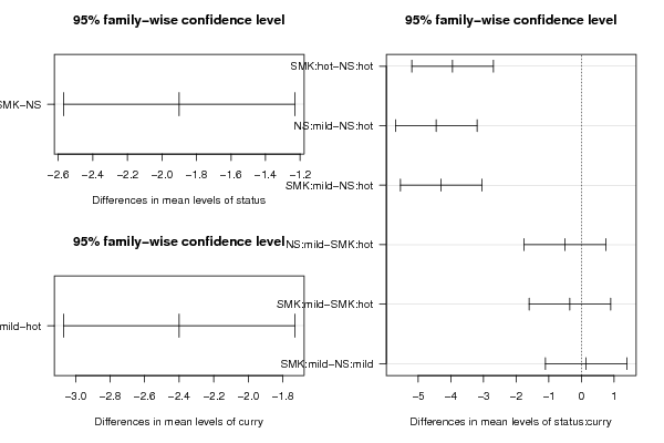
| Original text written by user: | Artificial data for demonstration of ANOVA | ||||||||||||||||||||||||||||||||||||||||||||||||||||||||||||||||||||||||||||||||||||||||||||||||||||||||||||||||||||||||||||||||||||||||||||||||||||||||||||||||||||||||||||||||||||||||||||||||||||||||||||||||||||||||||||||||||||||||||||||||||||||||||||||||||||||||||
| IsPrivate? | No (this computation is public) | ||||||||||||||||||||||||||||||||||||||||||||||||||||||||||||||||||||||||||||||||||||||||||||||||||||||||||||||||||||||||||||||||||||||||||||||||||||||||||||||||||||||||||||||||||||||||||||||||||||||||||||||||||||||||||||||||||||||||||||||||||||||||||||||||||||||||||
| User-defined keywords | |||||||||||||||||||||||||||||||||||||||||||||||||||||||||||||||||||||||||||||||||||||||||||||||||||||||||||||||||||||||||||||||||||||||||||||||||||||||||||||||||||||||||||||||||||||||||||||||||||||||||||||||||||||||||||||||||||||||||||||||||||||||||||||||||||||||||||
| Estimated Impact | 1142 | ||||||||||||||||||||||||||||||||||||||||||||||||||||||||||||||||||||||||||||||||||||||||||||||||||||||||||||||||||||||||||||||||||||||||||||||||||||||||||||||||||||||||||||||||||||||||||||||||||||||||||||||||||||||||||||||||||||||||||||||||||||||||||||||||||||||||||
Tree of Dependent Computations | |||||||||||||||||||||||||||||||||||||||||||||||||||||||||||||||||||||||||||||||||||||||||||||||||||||||||||||||||||||||||||||||||||||||||||||||||||||||||||||||||||||||||||||||||||||||||||||||||||||||||||||||||||||||||||||||||||||||||||||||||||||||||||||||||||||||||||
| Family? (F = Feedback message, R = changed R code, M = changed R Module, P = changed Parameters, D = changed Data) | |||||||||||||||||||||||||||||||||||||||||||||||||||||||||||||||||||||||||||||||||||||||||||||||||||||||||||||||||||||||||||||||||||||||||||||||||||||||||||||||||||||||||||||||||||||||||||||||||||||||||||||||||||||||||||||||||||||||||||||||||||||||||||||||||||||||||||
| - [Variability] [Two-Way ANOVA] [2010-11-30 21:42:30] [74be16979710d4c4e7c6647856088456] - RM [Two-Way ANOVA] [Two-Way ANOVA - C...] [2011-11-28 17:22:56] [a9208f4f8d3b118336aae915785f2bd9] [Current] - R [Two-Way ANOVA] [ANOVA Week 9] [2011-12-01 12:02:11] [0e3849a58d2010f680210bfa36dadcb4] - R [Two-Way ANOVA] [] [2011-12-01 12:02:56] [483074838c7eb9e0ff7f7d3e3c3f8586] - R [Two-Way ANOVA] [Question i] [2011-12-01 12:10:19] [57084a6890c0bc671c16163e98194e4e] - R [Two-Way ANOVA] [Spiciness Ratings] [2011-12-01 12:12:22] [68da2a3ec537521c4857f5c0bd5ed145] - RM [Two-Way ANOVA] [Compendium Week 9] [2011-12-01 12:08:25] [895f9de29a654334f7aa22b48b6b79ac] - RMPD [Histogram, QQplot and Density] [] [2011-12-01 12:13:45] [483074838c7eb9e0ff7f7d3e3c3f8586] - RMPD [Histogram, QQplot and Density] [Non smokers score...] [2011-12-01 12:15:07] [483074838c7eb9e0ff7f7d3e3c3f8586] - D [Histogram, QQplot and Density] [] [2011-12-01 12:21:02] [483074838c7eb9e0ff7f7d3e3c3f8586] - D [Histogram, QQplot and Density] [] [2011-12-01 12:23:01] [483074838c7eb9e0ff7f7d3e3c3f8586] - D [Histogram, QQplot and Density] [] [2011-12-01 12:33:41] [483074838c7eb9e0ff7f7d3e3c3f8586] - RMPD [Aston University Statistical Software] [] [2011-12-01 12:50:30] [483074838c7eb9e0ff7f7d3e3c3f8586] - R [Two-Way ANOVA] [] [2011-12-01 12:16:02] [e3bca26b0e60ee0c7c12e4668b30341a] - R D [Two-Way ANOVA] [] [2011-12-01 12:16:50] [84f9d24ffbb976b91a97c3ec996667ce] - RMPD [Histogram, QQplot and Density] [] [2011-12-01 12:19:14] [84f9d24ffbb976b91a97c3ec996667ce] - R PD [Histogram, QQplot and Density] [Spiciness Ratings...] [2011-12-01 12:40:24] [84f9d24ffbb976b91a97c3ec996667ce] - R D [Histogram, QQplot and Density] [] [2011-12-04 14:48:16] [74be16979710d4c4e7c6647856088456] - R PD [Histogram, QQplot and Density] [] [2011-12-04 14:51:41] [74be16979710d4c4e7c6647856088456] - R PD [Histogram, QQplot and Density] [] [2011-12-04 14:52:21] [74be16979710d4c4e7c6647856088456] - R PD [Histogram, QQplot and Density] [] [2011-12-04 14:53:01] [74be16979710d4c4e7c6647856088456] - RM [Two-Way ANOVA] [boxplots week 9] [2011-12-01 12:16:52] [6c7941ad1a28776e0a3d3478d8e8be50] - RMP [Histogram, QQplot and Density] [example] [2011-12-01 12:19:02] [57084a6890c0bc671c16163e98194e4e] - R [Two-Way ANOVA] [Week 9] [2011-12-01 12:20:42] [4d6fcff7a029721f667cce838c3bc5ec] - RM [Two-Way ANOVA] [] [2011-12-01 12:20:43] [6920cf7129d32b5e1d3344311b2c82d4] - R [Two-Way ANOVA] [smoker?/curry sta...] [2011-12-01 12:20:56] [bf6019510b5bcef0d7dc6b5e3f13759f] - RM [Two-Way ANOVA] [Results for the e...] [2011-12-01 12:17:37] [454fdeac8293fa9258db047c8915ceb3] - RM [Two-Way ANOVA] [histogram and box...] [2011-12-01 12:25:24] [04881406e92e7b483917daebdd502463] - R [Two-Way ANOVA] [Boxplot for spici...] [2011-12-01 12:26:54] [553711af6a3a99aac240956ee7ba8417] - RMPD [Histogram, QQplot and Density] [histogram rating] [2011-12-01 12:27:18] [bee56a896f26c17646228a77f17a2aff] - RMPD [Boxplot and Trimmed Means] [box plot smoker n...] [2011-12-01 12:44:04] [bee56a896f26c17646228a77f17a2aff] - R [Two-Way ANOVA] [2 way ANOVA for c...] [2011-12-01 12:32:55] [c2d7eae68f5ec0337d2d2ba826377ba0] - RM [Two-Way ANOVA] [W9 Two way ANOVA ...] [2011-12-01 12:33:10] [5af04e13c06bbf1f7fb207eb9550d664] - RM [Two-Way ANOVA] [comp 9] [2011-12-01 12:33:04] [d2893370a6bab19f4850e41a1f5affd5] - RM D [Histogram, QQplot and Density] [smokers rating of...] [2011-12-01 12:34:37] [e3bca26b0e60ee0c7c12e4668b30341a] - R D [Histogram, QQplot and Density] [smokers and korma...] [2011-12-01 12:37:15] [e3bca26b0e60ee0c7c12e4668b30341a] - D [Histogram, QQplot and Density] [non smokers vindaloo] [2011-12-01 12:39:42] [e3bca26b0e60ee0c7c12e4668b30341a] - D [Histogram, QQplot and Density] [non smokers korma] [2011-12-01 12:41:41] [e3bca26b0e60ee0c7c12e4668b30341a] - R P [Histogram, QQplot and Density] [Yoddlee] [2012-11-21 10:15:37] [74be16979710d4c4e7c6647856088456] - RMP [Histogram, QQplot and Density] [Compendium Week 9 ] [2011-12-01 12:34:40] [895f9de29a654334f7aa22b48b6b79ac] - RM [Two-Way ANOVA] [histogrm week 9 ] [2011-12-01 12:36:51] [39ce388efffdeef2308177e33597aa30] - R [Two-Way ANOVA] [Checking for homo...] [2011-12-01 12:38:37] [bdeb1591ecf7a4fb2b8ebb6101b513c3] - R P [Two-Way ANOVA] [Rating of hotness...] [2011-12-01 12:41:17] [a7ea7f4263337445a0a4c6547fb2278a] - RMPD [Notched Boxplots] [Spiciness box plot] [2011-12-01 12:36:29] [8be39d68cf3e859c626e6f1d2306767c] - RMP [Histogram, QQplot and Density] [] [2011-12-01 12:44:10] [6920cf7129d32b5e1d3344311b2c82d4] - RM [Two-Way ANOVA] [2 way ANOVA] [2011-12-01 12:45:02] [e3bca26b0e60ee0c7c12e4668b30341a] - RM [Two-Way ANOVA] [Blog] [2011-12-01 12:48:43] [eaa1051df62e3cae1e5cf7c042ac8911] - R D [Two-Way ANOVA] [curry vs smoker v...] [2011-12-01 12:45:19] [74be16979710d4c4e7c6647856088456] - R D [Two-Way ANOVA] [] [2011-12-01 12:45:19] [74be16979710d4c4e7c6647856088456] - RM [Two-Way ANOVA] [] [2011-12-01 12:49:55] [db1d7c04a949ca0eb268b1942f189a57] [Truncated] | |||||||||||||||||||||||||||||||||||||||||||||||||||||||||||||||||||||||||||||||||||||||||||||||||||||||||||||||||||||||||||||||||||||||||||||||||||||||||||||||||||||||||||||||||||||||||||||||||||||||||||||||||||||||||||||||||||||||||||||||||||||||||||||||||||||||||||
| Feedback Forum | |||||||||||||||||||||||||||||||||||||||||||||||||||||||||||||||||||||||||||||||||||||||||||||||||||||||||||||||||||||||||||||||||||||||||||||||||||||||||||||||||||||||||||||||||||||||||||||||||||||||||||||||||||||||||||||||||||||||||||||||||||||||||||||||||||||||||||
Post a new message | |||||||||||||||||||||||||||||||||||||||||||||||||||||||||||||||||||||||||||||||||||||||||||||||||||||||||||||||||||||||||||||||||||||||||||||||||||||||||||||||||||||||||||||||||||||||||||||||||||||||||||||||||||||||||||||||||||||||||||||||||||||||||||||||||||||||||||
Dataset | |||||||||||||||||||||||||||||||||||||||||||||||||||||||||||||||||||||||||||||||||||||||||||||||||||||||||||||||||||||||||||||||||||||||||||||||||||||||||||||||||||||||||||||||||||||||||||||||||||||||||||||||||||||||||||||||||||||||||||||||||||||||||||||||||||||||||||
| Dataseries X: | |||||||||||||||||||||||||||||||||||||||||||||||||||||||||||||||||||||||||||||||||||||||||||||||||||||||||||||||||||||||||||||||||||||||||||||||||||||||||||||||||||||||||||||||||||||||||||||||||||||||||||||||||||||||||||||||||||||||||||||||||||||||||||||||||||||||||||
4 'SMK' 'hot' 5 'SMK' 'hot' 3 'SMK' 'hot' 4 'SMK' 'hot' 5 'SMK' 'hot' 3 'SMK' 'hot' 7 'SMK' 'hot' 5 'SMK' 'hot' 6 'SMK' 'hot' 3 'SMK' 'hot' 2 'SMK' 'hot' 4 'SMK' 'hot' 5 'SMK' 'hot' 2 'SMK' 'hot' 3 'SMK' 'hot' 6 'SMK' 'hot' 4 'SMK' 'hot' 4 'SMK' 'hot' 6 'SMK' 'hot' 2 'SMK' 'hot' 3 'SMK' 'mild' 5 'SMK' 'mild' 4 'SMK' 'mild' 2 'SMK' 'mild' 7 'SMK' 'mild' 1 'SMK' 'mild' 4 'SMK' 'mild' 4 'SMK' 'mild' 7 'SMK' 'mild' 4 'SMK' 'mild' 3 'SMK' 'mild' 3 'SMK' 'mild' 3 'SMK' 'mild' 3 'SMK' 'mild' 2 'SMK' 'mild' 5 'SMK' 'mild' 5 'SMK' 'mild' 3 'SMK' 'mild' 6 'SMK' 'mild' 2 'SMK' 'mild' 8 'NS' 'hot' 9 'NS' 'hot' 10 'NS' 'hot' 7 'NS' 'hot' 8 'NS' 'hot' 9 'NS' 'hot' 10 'NS' 'hot' 6 'NS' 'hot' 6 'NS' 'hot' 7 'NS' 'hot' 8 'NS' 'hot' 9 'NS' 'hot' 8 'NS' 'hot' 7 'NS' 'hot' 5 'NS' 'hot' 11 'NS' 'hot' 7 'NS' 'hot' 8 'NS' 'hot' 10 'NS' 'hot' 9 'NS' 'hot' 3 'NS' 'mild' 5 'NS' 'mild' 4 'NS' 'mild' 2 'NS' 'mild' 6 'NS' 'mild' 1 'NS' 'mild' 4 'NS' 'mild' 4 'NS' 'mild' 5 'NS' 'mild' 4 'NS' 'mild' 3 'NS' 'mild' 3 'NS' 'mild' 4 'NS' 'mild' 3 'NS' 'mild' 2 'NS' 'mild' 5 'NS' 'mild' 4 'NS' 'mild' 3 'NS' 'mild' 6 'NS' 'mild' 2 'NS' 'mild' | |||||||||||||||||||||||||||||||||||||||||||||||||||||||||||||||||||||||||||||||||||||||||||||||||||||||||||||||||||||||||||||||||||||||||||||||||||||||||||||||||||||||||||||||||||||||||||||||||||||||||||||||||||||||||||||||||||||||||||||||||||||||||||||||||||||||||||
Tables (Output of Computation) | |||||||||||||||||||||||||||||||||||||||||||||||||||||||||||||||||||||||||||||||||||||||||||||||||||||||||||||||||||||||||||||||||||||||||||||||||||||||||||||||||||||||||||||||||||||||||||||||||||||||||||||||||||||||||||||||||||||||||||||||||||||||||||||||||||||||||||
| |||||||||||||||||||||||||||||||||||||||||||||||||||||||||||||||||||||||||||||||||||||||||||||||||||||||||||||||||||||||||||||||||||||||||||||||||||||||||||||||||||||||||||||||||||||||||||||||||||||||||||||||||||||||||||||||||||||||||||||||||||||||||||||||||||||||||||
Figures (Output of Computation) | |||||||||||||||||||||||||||||||||||||||||||||||||||||||||||||||||||||||||||||||||||||||||||||||||||||||||||||||||||||||||||||||||||||||||||||||||||||||||||||||||||||||||||||||||||||||||||||||||||||||||||||||||||||||||||||||||||||||||||||||||||||||||||||||||||||||||||
Input Parameters & R Code | |||||||||||||||||||||||||||||||||||||||||||||||||||||||||||||||||||||||||||||||||||||||||||||||||||||||||||||||||||||||||||||||||||||||||||||||||||||||||||||||||||||||||||||||||||||||||||||||||||||||||||||||||||||||||||||||||||||||||||||||||||||||||||||||||||||||||||
| Parameters (Session): | |||||||||||||||||||||||||||||||||||||||||||||||||||||||||||||||||||||||||||||||||||||||||||||||||||||||||||||||||||||||||||||||||||||||||||||||||||||||||||||||||||||||||||||||||||||||||||||||||||||||||||||||||||||||||||||||||||||||||||||||||||||||||||||||||||||||||||
| par1 = 1 ; par2 = 2 ; par3 = 3 ; par4 = TRUE ; | |||||||||||||||||||||||||||||||||||||||||||||||||||||||||||||||||||||||||||||||||||||||||||||||||||||||||||||||||||||||||||||||||||||||||||||||||||||||||||||||||||||||||||||||||||||||||||||||||||||||||||||||||||||||||||||||||||||||||||||||||||||||||||||||||||||||||||
| Parameters (R input): | |||||||||||||||||||||||||||||||||||||||||||||||||||||||||||||||||||||||||||||||||||||||||||||||||||||||||||||||||||||||||||||||||||||||||||||||||||||||||||||||||||||||||||||||||||||||||||||||||||||||||||||||||||||||||||||||||||||||||||||||||||||||||||||||||||||||||||
| par1 = 1 ; par2 = 2 ; par3 = 3 ; par4 = TRUE ; | |||||||||||||||||||||||||||||||||||||||||||||||||||||||||||||||||||||||||||||||||||||||||||||||||||||||||||||||||||||||||||||||||||||||||||||||||||||||||||||||||||||||||||||||||||||||||||||||||||||||||||||||||||||||||||||||||||||||||||||||||||||||||||||||||||||||||||
| R code (references can be found in the software module): | |||||||||||||||||||||||||||||||||||||||||||||||||||||||||||||||||||||||||||||||||||||||||||||||||||||||||||||||||||||||||||||||||||||||||||||||||||||||||||||||||||||||||||||||||||||||||||||||||||||||||||||||||||||||||||||||||||||||||||||||||||||||||||||||||||||||||||
cat1 <- as.numeric(par1) # | |||||||||||||||||||||||||||||||||||||||||||||||||||||||||||||||||||||||||||||||||||||||||||||||||||||||||||||||||||||||||||||||||||||||||||||||||||||||||||||||||||||||||||||||||||||||||||||||||||||||||||||||||||||||||||||||||||||||||||||||||||||||||||||||||||||||||||