Repository of Reproducible Computations

Free Statistics

of Irreproducible Research!

Author's title

Author

*The author of this computation has been verified*

R Software Module

rwasp_autocorrelation.wasp

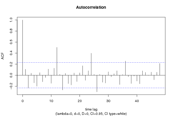
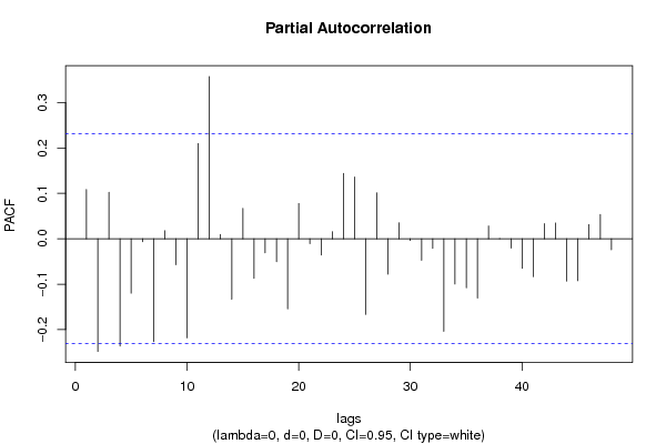
Title produced by software

(Partial) Autocorrelation Function

Date of computation

Tue, 06 Dec 2011 16:39:45 -0500

Cite this page as follows

Statistical Computations at FreeStatistics.org, Office for Research Development and Education, URL https://freestatistics.org/blog/index.php?v=date/2011/Dec/06/t1323207605xffnt23rvzfcw8s.htm/, Retrieved Sun, 28 Apr 2024 22:38:02 +0000

Statistical Computations at FreeStatistics.org, Office for Research Development and Education, URL https://freestatistics.org/blog/index.php?pk=151966, Retrieved Sun, 28 Apr 2024 22:38:02 +0000

QR Codes:

Paste this QR Code to cite your computation.

Original text written by user:

IsPrivate?

No (this computation is public)

User-defined keywords

Estimated Impact

Family? (F = Feedback message, R = changed R code, M = changed R Module, P = changed Parameters, D = changed Data)

-     [Univariate Data Series] [] [2008-12-14 11:54:22] [d2d412c7f4d35ffbf5ee5ee89db327d4]
- RMP     [(Partial) Autocorrelation Function] [1] [2011-12-06 21:39:45] [0652e0694c2cbf138ee0a1c8d686a8e4] [Current]
- R P       [(Partial) Autocorrelation Function] [2] [2011-12-06 21:42:43] [98f3ba974ec9d6d754dcc83206539a91] 
- RMP       [Spectral Analysis] [3] [2011-12-06 21:46:09] [98f3ba974ec9d6d754dcc83206539a91] 
-   P         [Spectral Analysis] [5] [2011-12-07 06:02:14] [98f3ba974ec9d6d754dcc83206539a91] 
- RMP           [Standard Deviation-Mean Plot] [6] [2011-12-07 06:05:38] [98f3ba974ec9d6d754dcc83206539a91] 
- RMP           [Variance Reduction Matrix] [7] [2011-12-07 07:11:48] [98f3ba974ec9d6d754dcc83206539a91] 

Feedback Forum

Post a new message

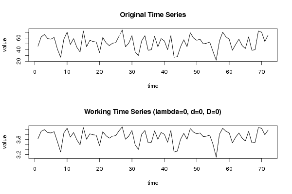
Dataseries X:

Download CSV

Histogram

Boxplots

Summary of computational transaction
Raw Input	view raw input (R code)
Raw Output	view raw output of R engine
Computing time	1 seconds
R Server	'Gwilym Jenkins' @ jenkins.wessa.net

\begin{tabular}{lllllllll}
\hline
Summary of computational transaction \tabularnewline
Raw Input & view raw input (R code)  \tabularnewline
Raw Output & view raw output of R engine  \tabularnewline
Computing time & 1 seconds \tabularnewline
R Server & 'Gwilym Jenkins' @ jenkins.wessa.net \tabularnewline
\hline
\end{tabular}
%Source: https://freestatistics.org/blog/index.php?pk=151966&T=0

[TABLE]
[ROW][C]Summary of computational transaction[/C][/ROW]
[ROW][C]Raw Input[/C][C]view raw input (R code) [/C][/ROW]
[ROW][C]Raw Output[/C][C]view raw output of R engine [/C][/ROW]
[ROW][C]Computing time[/C][C]1 seconds[/C][/ROW]
[ROW][C]R Server[/C][C]'Gwilym Jenkins' @ jenkins.wessa.net[/C][/ROW]
[/TABLE]
Source: https://freestatistics.org/blog/index.php?pk=151966&T=0

Globally Unique Identifier (entire table): ba.freestatistics.org/blog/index.php?pk=151966&T=0

As an alternative you can also use a QR Code:

The GUIDs for individual cells are displayed in the table below:

Summary of computational transaction
Raw Input	view raw input (R code)
Raw Output	view raw output of R engine
Computing time	1 seconds
R Server	'Gwilym Jenkins' @ jenkins.wessa.net

Autocorrelation Function
Time lag k	ACF(k)	T-STAT	P-value
1	0.10831	0.919	0.180572
2	-0.233642	-1.9825	0.025619
3	0.036615	0.3107	0.378468
4	-0.138675	-1.1767	0.121596
5	-0.199834	-1.6957	0.047136
6	0.046609	0.3955	0.346826
7	-0.119509	-1.0141	0.156974
8	-0.041871	-0.3553	0.361705
9	0.110718	0.9395	0.175314
10	-0.146997	-1.2473	0.108163
11	0.12665	1.0747	0.143057
12	0.504361	4.2796	2.8e-05
13	0.013827	0.1173	0.453463
14	-0.267883	-2.2731	0.013004
15	0.03335	0.283	0.389001
16	-0.152685	-1.2956	0.09963
17	-0.177306	-1.5045	0.068415
18	0.040431	0.3431	0.366275
19	-0.115608	-0.981	0.164947
20	0.042942	0.3644	0.358323
21	0.171289	1.4534	0.075224
22	-0.093635	-0.7945	0.214751
23	0.080193	0.6805	0.249199
24	0.398251	3.3793	0.000588
25	0.014129	0.1199	0.452451
26	-0.301481	-2.5581	0.006314
27	0.0129	0.1095	0.456572
28	-0.128353	-1.0891	0.139868
29	-0.141662	-1.202	0.116643
30	0.060625	0.5144	0.304266
31	-0.029614	-0.2513	0.401157
32	0.026301	0.2232	0.412017
33	0.080261	0.681	0.249017
34	-0.169368	-1.4371	0.077506
35	0.010329	0.0876	0.465201
36	0.256989	2.1806	0.01624
37	-0.02623	-0.2226	0.41225
38	-0.151122	-1.2823	0.101923
39	-0.014997	-0.1272	0.449549
40	-0.106558	-0.9042	0.184459
41	-0.15559	-1.3202	0.095471
42	0.07865	0.6674	0.253336
43	0.051164	0.4341	0.332741
44	-0.004179	-0.0355	0.485904
45	0.055581	0.4716	0.319311
46	-0.083461	-0.7082	0.240558
47	0.053388	0.453	0.325952
48	0.21245	1.8027	0.03781

\begin{tabular}{lllllllll}
\hline
Autocorrelation Function \tabularnewline
Time lag k & ACF(k) & T-STAT & P-value \tabularnewline
1 & 0.10831 & 0.919 & 0.180572 \tabularnewline
2 & -0.233642 & -1.9825 & 0.025619 \tabularnewline
3 & 0.036615 & 0.3107 & 0.378468 \tabularnewline
4 & -0.138675 & -1.1767 & 0.121596 \tabularnewline
5 & -0.199834 & -1.6957 & 0.047136 \tabularnewline
6 & 0.046609 & 0.3955 & 0.346826 \tabularnewline
7 & -0.119509 & -1.0141 & 0.156974 \tabularnewline
8 & -0.041871 & -0.3553 & 0.361705 \tabularnewline
9 & 0.110718 & 0.9395 & 0.175314 \tabularnewline
10 & -0.146997 & -1.2473 & 0.108163 \tabularnewline
11 & 0.12665 & 1.0747 & 0.143057 \tabularnewline
12 & 0.504361 & 4.2796 & 2.8e-05 \tabularnewline
13 & 0.013827 & 0.1173 & 0.453463 \tabularnewline
14 & -0.267883 & -2.2731 & 0.013004 \tabularnewline
15 & 0.03335 & 0.283 & 0.389001 \tabularnewline
16 & -0.152685 & -1.2956 & 0.09963 \tabularnewline
17 & -0.177306 & -1.5045 & 0.068415 \tabularnewline
18 & 0.040431 & 0.3431 & 0.366275 \tabularnewline
19 & -0.115608 & -0.981 & 0.164947 \tabularnewline
20 & 0.042942 & 0.3644 & 0.358323 \tabularnewline
21 & 0.171289 & 1.4534 & 0.075224 \tabularnewline
22 & -0.093635 & -0.7945 & 0.214751 \tabularnewline
23 & 0.080193 & 0.6805 & 0.249199 \tabularnewline
24 & 0.398251 & 3.3793 & 0.000588 \tabularnewline
25 & 0.014129 & 0.1199 & 0.452451 \tabularnewline
26 & -0.301481 & -2.5581 & 0.006314 \tabularnewline
27 & 0.0129 & 0.1095 & 0.456572 \tabularnewline
28 & -0.128353 & -1.0891 & 0.139868 \tabularnewline
29 & -0.141662 & -1.202 & 0.116643 \tabularnewline
30 & 0.060625 & 0.5144 & 0.304266 \tabularnewline
31 & -0.029614 & -0.2513 & 0.401157 \tabularnewline
32 & 0.026301 & 0.2232 & 0.412017 \tabularnewline
33 & 0.080261 & 0.681 & 0.249017 \tabularnewline
34 & -0.169368 & -1.4371 & 0.077506 \tabularnewline
35 & 0.010329 & 0.0876 & 0.465201 \tabularnewline
36 & 0.256989 & 2.1806 & 0.01624 \tabularnewline
37 & -0.02623 & -0.2226 & 0.41225 \tabularnewline
38 & -0.151122 & -1.2823 & 0.101923 \tabularnewline
39 & -0.014997 & -0.1272 & 0.449549 \tabularnewline
40 & -0.106558 & -0.9042 & 0.184459 \tabularnewline
41 & -0.15559 & -1.3202 & 0.095471 \tabularnewline
42 & 0.07865 & 0.6674 & 0.253336 \tabularnewline
43 & 0.051164 & 0.4341 & 0.332741 \tabularnewline
44 & -0.004179 & -0.0355 & 0.485904 \tabularnewline
45 & 0.055581 & 0.4716 & 0.319311 \tabularnewline
46 & -0.083461 & -0.7082 & 0.240558 \tabularnewline
47 & 0.053388 & 0.453 & 0.325952 \tabularnewline
48 & 0.21245 & 1.8027 & 0.03781 \tabularnewline
\hline
\end{tabular}
%Source: https://freestatistics.org/blog/index.php?pk=151966&T=1

[TABLE]
[ROW][C]Autocorrelation Function[/C][/ROW]
[ROW][C]Time lag k[/C][C]ACF(k)[/C][C]T-STAT[/C][C]P-value[/C][/ROW]
[ROW][C]1[/C][C]0.10831[/C][C]0.919[/C][C]0.180572[/C][/ROW]
[ROW][C]2[/C][C]-0.233642[/C][C]-1.9825[/C][C]0.025619[/C][/ROW]
[ROW][C]3[/C][C]0.036615[/C][C]0.3107[/C][C]0.378468[/C][/ROW]
[ROW][C]4[/C][C]-0.138675[/C][C]-1.1767[/C][C]0.121596[/C][/ROW]
[ROW][C]5[/C][C]-0.199834[/C][C]-1.6957[/C][C]0.047136[/C][/ROW]
[ROW][C]6[/C][C]0.046609[/C][C]0.3955[/C][C]0.346826[/C][/ROW]
[ROW][C]7[/C][C]-0.119509[/C][C]-1.0141[/C][C]0.156974[/C][/ROW]
[ROW][C]8[/C][C]-0.041871[/C][C]-0.3553[/C][C]0.361705[/C][/ROW]
[ROW][C]9[/C][C]0.110718[/C][C]0.9395[/C][C]0.175314[/C][/ROW]
[ROW][C]10[/C][C]-0.146997[/C][C]-1.2473[/C][C]0.108163[/C][/ROW]
[ROW][C]11[/C][C]0.12665[/C][C]1.0747[/C][C]0.143057[/C][/ROW]
[ROW][C]12[/C][C]0.504361[/C][C]4.2796[/C][C]2.8e-05[/C][/ROW]
[ROW][C]13[/C][C]0.013827[/C][C]0.1173[/C][C]0.453463[/C][/ROW]
[ROW][C]14[/C][C]-0.267883[/C][C]-2.2731[/C][C]0.013004[/C][/ROW]
[ROW][C]15[/C][C]0.03335[/C][C]0.283[/C][C]0.389001[/C][/ROW]
[ROW][C]16[/C][C]-0.152685[/C][C]-1.2956[/C][C]0.09963[/C][/ROW]
[ROW][C]17[/C][C]-0.177306[/C][C]-1.5045[/C][C]0.068415[/C][/ROW]
[ROW][C]18[/C][C]0.040431[/C][C]0.3431[/C][C]0.366275[/C][/ROW]
[ROW][C]19[/C][C]-0.115608[/C][C]-0.981[/C][C]0.164947[/C][/ROW]
[ROW][C]20[/C][C]0.042942[/C][C]0.3644[/C][C]0.358323[/C][/ROW]
[ROW][C]21[/C][C]0.171289[/C][C]1.4534[/C][C]0.075224[/C][/ROW]
[ROW][C]22[/C][C]-0.093635[/C][C]-0.7945[/C][C]0.214751[/C][/ROW]
[ROW][C]23[/C][C]0.080193[/C][C]0.6805[/C][C]0.249199[/C][/ROW]
[ROW][C]24[/C][C]0.398251[/C][C]3.3793[/C][C]0.000588[/C][/ROW]
[ROW][C]25[/C][C]0.014129[/C][C]0.1199[/C][C]0.452451[/C][/ROW]
[ROW][C]26[/C][C]-0.301481[/C][C]-2.5581[/C][C]0.006314[/C][/ROW]
[ROW][C]27[/C][C]0.0129[/C][C]0.1095[/C][C]0.456572[/C][/ROW]
[ROW][C]28[/C][C]-0.128353[/C][C]-1.0891[/C][C]0.139868[/C][/ROW]
[ROW][C]29[/C][C]-0.141662[/C][C]-1.202[/C][C]0.116643[/C][/ROW]
[ROW][C]30[/C][C]0.060625[/C][C]0.5144[/C][C]0.304266[/C][/ROW]
[ROW][C]31[/C][C]-0.029614[/C][C]-0.2513[/C][C]0.401157[/C][/ROW]
[ROW][C]32[/C][C]0.026301[/C][C]0.2232[/C][C]0.412017[/C][/ROW]
[ROW][C]33[/C][C]0.080261[/C][C]0.681[/C][C]0.249017[/C][/ROW]
[ROW][C]34[/C][C]-0.169368[/C][C]-1.4371[/C][C]0.077506[/C][/ROW]
[ROW][C]35[/C][C]0.010329[/C][C]0.0876[/C][C]0.465201[/C][/ROW]
[ROW][C]36[/C][C]0.256989[/C][C]2.1806[/C][C]0.01624[/C][/ROW]
[ROW][C]37[/C][C]-0.02623[/C][C]-0.2226[/C][C]0.41225[/C][/ROW]
[ROW][C]38[/C][C]-0.151122[/C][C]-1.2823[/C][C]0.101923[/C][/ROW]
[ROW][C]39[/C][C]-0.014997[/C][C]-0.1272[/C][C]0.449549[/C][/ROW]
[ROW][C]40[/C][C]-0.106558[/C][C]-0.9042[/C][C]0.184459[/C][/ROW]
[ROW][C]41[/C][C]-0.15559[/C][C]-1.3202[/C][C]0.095471[/C][/ROW]
[ROW][C]42[/C][C]0.07865[/C][C]0.6674[/C][C]0.253336[/C][/ROW]
[ROW][C]43[/C][C]0.051164[/C][C]0.4341[/C][C]0.332741[/C][/ROW]
[ROW][C]44[/C][C]-0.004179[/C][C]-0.0355[/C][C]0.485904[/C][/ROW]
[ROW][C]45[/C][C]0.055581[/C][C]0.4716[/C][C]0.319311[/C][/ROW]
[ROW][C]46[/C][C]-0.083461[/C][C]-0.7082[/C][C]0.240558[/C][/ROW]
[ROW][C]47[/C][C]0.053388[/C][C]0.453[/C][C]0.325952[/C][/ROW]
[ROW][C]48[/C][C]0.21245[/C][C]1.8027[/C][C]0.03781[/C][/ROW]
[/TABLE]
Source: https://freestatistics.org/blog/index.php?pk=151966&T=1

Globally Unique Identifier (entire table): ba.freestatistics.org/blog/index.php?pk=151966&T=1

As an alternative you can also use a QR Code:

The GUIDs for individual cells are displayed in the table below:

Autocorrelation Function
Time lag k	ACF(k)	T-STAT	P-value
1	0.10831	0.919	0.180572
2	-0.233642	-1.9825	0.025619
3	0.036615	0.3107	0.378468
4	-0.138675	-1.1767	0.121596
5	-0.199834	-1.6957	0.047136
6	0.046609	0.3955	0.346826
7	-0.119509	-1.0141	0.156974
8	-0.041871	-0.3553	0.361705
9	0.110718	0.9395	0.175314
10	-0.146997	-1.2473	0.108163
11	0.12665	1.0747	0.143057
12	0.504361	4.2796	2.8e-05
13	0.013827	0.1173	0.453463
14	-0.267883	-2.2731	0.013004
15	0.03335	0.283	0.389001
16	-0.152685	-1.2956	0.09963
17	-0.177306	-1.5045	0.068415
18	0.040431	0.3431	0.366275
19	-0.115608	-0.981	0.164947
20	0.042942	0.3644	0.358323
21	0.171289	1.4534	0.075224
22	-0.093635	-0.7945	0.214751
23	0.080193	0.6805	0.249199
24	0.398251	3.3793	0.000588
25	0.014129	0.1199	0.452451
26	-0.301481	-2.5581	0.006314
27	0.0129	0.1095	0.456572
28	-0.128353	-1.0891	0.139868
29	-0.141662	-1.202	0.116643
30	0.060625	0.5144	0.304266
31	-0.029614	-0.2513	0.401157
32	0.026301	0.2232	0.412017
33	0.080261	0.681	0.249017
34	-0.169368	-1.4371	0.077506
35	0.010329	0.0876	0.465201
36	0.256989	2.1806	0.01624
37	-0.02623	-0.2226	0.41225
38	-0.151122	-1.2823	0.101923
39	-0.014997	-0.1272	0.449549
40	-0.106558	-0.9042	0.184459
41	-0.15559	-1.3202	0.095471
42	0.07865	0.6674	0.253336
43	0.051164	0.4341	0.332741
44	-0.004179	-0.0355	0.485904
45	0.055581	0.4716	0.319311
46	-0.083461	-0.7082	0.240558
47	0.053388	0.453	0.325952
48	0.21245	1.8027	0.03781

Partial Autocorrelation Function
Time lag k	PACF(k)	T-STAT	P-value
1	0.10831	0.919	0.180572
2	-0.248286	-2.1068	0.019311
3	0.102546	0.8701	0.193561
4	-0.236394	-2.0059	0.024314
5	-0.11992	-1.0176	0.156148
6	-0.006443	-0.0547	0.478276
7	-0.226544	-1.9223	0.029263
8	0.017647	0.1497	0.440694
9	-0.057326	-0.4864	0.314071
10	-0.218287	-1.8522	0.034047
11	0.209738	1.7797	0.039674
12	0.357377	3.0324	0.001686
13	0.00926	0.0786	0.468793
14	-0.133235	-1.1305	0.131001
15	0.066997	0.5685	0.285736
16	-0.086978	-0.738	0.231448
17	-0.030807	-0.2614	0.397263
18	-0.05047	-0.4283	0.334872
19	-0.154501	-1.311	0.097014
20	0.077612	0.6586	0.25614
21	-0.010907	-0.0926	0.463258
22	-0.035991	-0.3054	0.380474
23	0.015656	0.1328	0.447344
24	0.143743	1.2197	0.11328
25	0.135785	1.1522	0.126531
26	-0.166577	-1.4135	0.080916
27	0.101313	0.8597	0.196413
28	-0.077988	-0.6618	0.255122
29	0.035004	0.297	0.383653
30	-0.0037	-0.0314	0.48752
31	-0.047253	-0.401	0.344821
32	-0.020974	-0.178	0.429623
33	-0.204048	-1.7314	0.043832
34	-0.099742	-0.8463	0.200083
35	-0.107863	-0.9152	0.181559
36	-0.130625	-1.1084	0.135691
37	0.028198	0.2393	0.405789
38	-0.000421	-0.0036	0.498581
39	-0.020636	-0.1751	0.430744
40	-0.065332	-0.5544	0.290524
41	-0.083423	-0.7079	0.240655
42	0.033189	0.2816	0.389524
43	0.034747	0.2948	0.384484
44	-0.093307	-0.7917	0.215557
45	-0.092318	-0.7833	0.217996
46	0.03121	0.2648	0.395951
47	0.053302	0.4523	0.326213
48	-0.024403	-0.2071	0.418273

\begin{tabular}{lllllllll}
\hline
Partial Autocorrelation Function \tabularnewline
Time lag k & PACF(k) & T-STAT & P-value \tabularnewline
1 & 0.10831 & 0.919 & 0.180572 \tabularnewline
2 & -0.248286 & -2.1068 & 0.019311 \tabularnewline
3 & 0.102546 & 0.8701 & 0.193561 \tabularnewline
4 & -0.236394 & -2.0059 & 0.024314 \tabularnewline
5 & -0.11992 & -1.0176 & 0.156148 \tabularnewline
6 & -0.006443 & -0.0547 & 0.478276 \tabularnewline
7 & -0.226544 & -1.9223 & 0.029263 \tabularnewline
8 & 0.017647 & 0.1497 & 0.440694 \tabularnewline
9 & -0.057326 & -0.4864 & 0.314071 \tabularnewline
10 & -0.218287 & -1.8522 & 0.034047 \tabularnewline
11 & 0.209738 & 1.7797 & 0.039674 \tabularnewline
12 & 0.357377 & 3.0324 & 0.001686 \tabularnewline
13 & 0.00926 & 0.0786 & 0.468793 \tabularnewline
14 & -0.133235 & -1.1305 & 0.131001 \tabularnewline
15 & 0.066997 & 0.5685 & 0.285736 \tabularnewline
16 & -0.086978 & -0.738 & 0.231448 \tabularnewline
17 & -0.030807 & -0.2614 & 0.397263 \tabularnewline
18 & -0.05047 & -0.4283 & 0.334872 \tabularnewline
19 & -0.154501 & -1.311 & 0.097014 \tabularnewline
20 & 0.077612 & 0.6586 & 0.25614 \tabularnewline
21 & -0.010907 & -0.0926 & 0.463258 \tabularnewline
22 & -0.035991 & -0.3054 & 0.380474 \tabularnewline
23 & 0.015656 & 0.1328 & 0.447344 \tabularnewline
24 & 0.143743 & 1.2197 & 0.11328 \tabularnewline
25 & 0.135785 & 1.1522 & 0.126531 \tabularnewline
26 & -0.166577 & -1.4135 & 0.080916 \tabularnewline
27 & 0.101313 & 0.8597 & 0.196413 \tabularnewline
28 & -0.077988 & -0.6618 & 0.255122 \tabularnewline
29 & 0.035004 & 0.297 & 0.383653 \tabularnewline
30 & -0.0037 & -0.0314 & 0.48752 \tabularnewline
31 & -0.047253 & -0.401 & 0.344821 \tabularnewline
32 & -0.020974 & -0.178 & 0.429623 \tabularnewline
33 & -0.204048 & -1.7314 & 0.043832 \tabularnewline
34 & -0.099742 & -0.8463 & 0.200083 \tabularnewline
35 & -0.107863 & -0.9152 & 0.181559 \tabularnewline
36 & -0.130625 & -1.1084 & 0.135691 \tabularnewline
37 & 0.028198 & 0.2393 & 0.405789 \tabularnewline
38 & -0.000421 & -0.0036 & 0.498581 \tabularnewline
39 & -0.020636 & -0.1751 & 0.430744 \tabularnewline
40 & -0.065332 & -0.5544 & 0.290524 \tabularnewline
41 & -0.083423 & -0.7079 & 0.240655 \tabularnewline
42 & 0.033189 & 0.2816 & 0.389524 \tabularnewline
43 & 0.034747 & 0.2948 & 0.384484 \tabularnewline
44 & -0.093307 & -0.7917 & 0.215557 \tabularnewline
45 & -0.092318 & -0.7833 & 0.217996 \tabularnewline
46 & 0.03121 & 0.2648 & 0.395951 \tabularnewline
47 & 0.053302 & 0.4523 & 0.326213 \tabularnewline
48 & -0.024403 & -0.2071 & 0.418273 \tabularnewline
\hline
\end{tabular}
%Source: https://freestatistics.org/blog/index.php?pk=151966&T=2

[TABLE]
[ROW][C]Partial Autocorrelation Function[/C][/ROW]
[ROW][C]Time lag k[/C][C]PACF(k)[/C][C]T-STAT[/C][C]P-value[/C][/ROW]
[ROW][C]1[/C][C]0.10831[/C][C]0.919[/C][C]0.180572[/C][/ROW]
[ROW][C]2[/C][C]-0.248286[/C][C]-2.1068[/C][C]0.019311[/C][/ROW]
[ROW][C]3[/C][C]0.102546[/C][C]0.8701[/C][C]0.193561[/C][/ROW]
[ROW][C]4[/C][C]-0.236394[/C][C]-2.0059[/C][C]0.024314[/C][/ROW]
[ROW][C]5[/C][C]-0.11992[/C][C]-1.0176[/C][C]0.156148[/C][/ROW]
[ROW][C]6[/C][C]-0.006443[/C][C]-0.0547[/C][C]0.478276[/C][/ROW]
[ROW][C]7[/C][C]-0.226544[/C][C]-1.9223[/C][C]0.029263[/C][/ROW]
[ROW][C]8[/C][C]0.017647[/C][C]0.1497[/C][C]0.440694[/C][/ROW]
[ROW][C]9[/C][C]-0.057326[/C][C]-0.4864[/C][C]0.314071[/C][/ROW]
[ROW][C]10[/C][C]-0.218287[/C][C]-1.8522[/C][C]0.034047[/C][/ROW]
[ROW][C]11[/C][C]0.209738[/C][C]1.7797[/C][C]0.039674[/C][/ROW]
[ROW][C]12[/C][C]0.357377[/C][C]3.0324[/C][C]0.001686[/C][/ROW]
[ROW][C]13[/C][C]0.00926[/C][C]0.0786[/C][C]0.468793[/C][/ROW]
[ROW][C]14[/C][C]-0.133235[/C][C]-1.1305[/C][C]0.131001[/C][/ROW]
[ROW][C]15[/C][C]0.066997[/C][C]0.5685[/C][C]0.285736[/C][/ROW]
[ROW][C]16[/C][C]-0.086978[/C][C]-0.738[/C][C]0.231448[/C][/ROW]
[ROW][C]17[/C][C]-0.030807[/C][C]-0.2614[/C][C]0.397263[/C][/ROW]
[ROW][C]18[/C][C]-0.05047[/C][C]-0.4283[/C][C]0.334872[/C][/ROW]
[ROW][C]19[/C][C]-0.154501[/C][C]-1.311[/C][C]0.097014[/C][/ROW]
[ROW][C]20[/C][C]0.077612[/C][C]0.6586[/C][C]0.25614[/C][/ROW]
[ROW][C]21[/C][C]-0.010907[/C][C]-0.0926[/C][C]0.463258[/C][/ROW]
[ROW][C]22[/C][C]-0.035991[/C][C]-0.3054[/C][C]0.380474[/C][/ROW]
[ROW][C]23[/C][C]0.015656[/C][C]0.1328[/C][C]0.447344[/C][/ROW]
[ROW][C]24[/C][C]0.143743[/C][C]1.2197[/C][C]0.11328[/C][/ROW]
[ROW][C]25[/C][C]0.135785[/C][C]1.1522[/C][C]0.126531[/C][/ROW]
[ROW][C]26[/C][C]-0.166577[/C][C]-1.4135[/C][C]0.080916[/C][/ROW]
[ROW][C]27[/C][C]0.101313[/C][C]0.8597[/C][C]0.196413[/C][/ROW]
[ROW][C]28[/C][C]-0.077988[/C][C]-0.6618[/C][C]0.255122[/C][/ROW]
[ROW][C]29[/C][C]0.035004[/C][C]0.297[/C][C]0.383653[/C][/ROW]
[ROW][C]30[/C][C]-0.0037[/C][C]-0.0314[/C][C]0.48752[/C][/ROW]
[ROW][C]31[/C][C]-0.047253[/C][C]-0.401[/C][C]0.344821[/C][/ROW]
[ROW][C]32[/C][C]-0.020974[/C][C]-0.178[/C][C]0.429623[/C][/ROW]
[ROW][C]33[/C][C]-0.204048[/C][C]-1.7314[/C][C]0.043832[/C][/ROW]
[ROW][C]34[/C][C]-0.099742[/C][C]-0.8463[/C][C]0.200083[/C][/ROW]
[ROW][C]35[/C][C]-0.107863[/C][C]-0.9152[/C][C]0.181559[/C][/ROW]
[ROW][C]36[/C][C]-0.130625[/C][C]-1.1084[/C][C]0.135691[/C][/ROW]
[ROW][C]37[/C][C]0.028198[/C][C]0.2393[/C][C]0.405789[/C][/ROW]
[ROW][C]38[/C][C]-0.000421[/C][C]-0.0036[/C][C]0.498581[/C][/ROW]
[ROW][C]39[/C][C]-0.020636[/C][C]-0.1751[/C][C]0.430744[/C][/ROW]
[ROW][C]40[/C][C]-0.065332[/C][C]-0.5544[/C][C]0.290524[/C][/ROW]
[ROW][C]41[/C][C]-0.083423[/C][C]-0.7079[/C][C]0.240655[/C][/ROW]
[ROW][C]42[/C][C]0.033189[/C][C]0.2816[/C][C]0.389524[/C][/ROW]
[ROW][C]43[/C][C]0.034747[/C][C]0.2948[/C][C]0.384484[/C][/ROW]
[ROW][C]44[/C][C]-0.093307[/C][C]-0.7917[/C][C]0.215557[/C][/ROW]
[ROW][C]45[/C][C]-0.092318[/C][C]-0.7833[/C][C]0.217996[/C][/ROW]
[ROW][C]46[/C][C]0.03121[/C][C]0.2648[/C][C]0.395951[/C][/ROW]
[ROW][C]47[/C][C]0.053302[/C][C]0.4523[/C][C]0.326213[/C][/ROW]
[ROW][C]48[/C][C]-0.024403[/C][C]-0.2071[/C][C]0.418273[/C][/ROW]
[/TABLE]
Source: https://freestatistics.org/blog/index.php?pk=151966&T=2

Globally Unique Identifier (entire table): ba.freestatistics.org/blog/index.php?pk=151966&T=2

As an alternative you can also use a QR Code:

The GUIDs for individual cells are displayed in the table below:

Partial Autocorrelation Function
Time lag k	PACF(k)	T-STAT	P-value
1	0.10831	0.919	0.180572
2	-0.248286	-2.1068	0.019311
3	0.102546	0.8701	0.193561
4	-0.236394	-2.0059	0.024314
5	-0.11992	-1.0176	0.156148
6	-0.006443	-0.0547	0.478276
7	-0.226544	-1.9223	0.029263
8	0.017647	0.1497	0.440694
9	-0.057326	-0.4864	0.314071
10	-0.218287	-1.8522	0.034047
11	0.209738	1.7797	0.039674
12	0.357377	3.0324	0.001686
13	0.00926	0.0786	0.468793
14	-0.133235	-1.1305	0.131001
15	0.066997	0.5685	0.285736
16	-0.086978	-0.738	0.231448
17	-0.030807	-0.2614	0.397263
18	-0.05047	-0.4283	0.334872
19	-0.154501	-1.311	0.097014
20	0.077612	0.6586	0.25614
21	-0.010907	-0.0926	0.463258
22	-0.035991	-0.3054	0.380474
23	0.015656	0.1328	0.447344
24	0.143743	1.2197	0.11328
25	0.135785	1.1522	0.126531
26	-0.166577	-1.4135	0.080916
27	0.101313	0.8597	0.196413
28	-0.077988	-0.6618	0.255122
29	0.035004	0.297	0.383653
30	-0.0037	-0.0314	0.48752
31	-0.047253	-0.401	0.344821
32	-0.020974	-0.178	0.429623
33	-0.204048	-1.7314	0.043832
34	-0.099742	-0.8463	0.200083
35	-0.107863	-0.9152	0.181559
36	-0.130625	-1.1084	0.135691
37	0.028198	0.2393	0.405789
38	-0.000421	-0.0036	0.498581
39	-0.020636	-0.1751	0.430744
40	-0.065332	-0.5544	0.290524
41	-0.083423	-0.7079	0.240655
42	0.033189	0.2816	0.389524
43	0.034747	0.2948	0.384484
44	-0.093307	-0.7917	0.215557
45	-0.092318	-0.7833	0.217996
46	0.03121	0.2648	0.395951
47	0.053302	0.4523	0.326213
48	-0.024403	-0.2071	0.418273

Figure 1

PNG link

Postscript link

PDF link

Figure 2

PNG link

Postscript link

PDF link

Figure 3

PNG link

Postscript link

PDF link

Parameters (Session):

par1 = 48 ; par2 = 0.0 ; par3 = 0 ; par4 = 0 ; par5 = 12 ; par6 = White Noise ; par7 = 0.95 ;

Parameters (R input):

par1 = 48 ; par2 = 0.0 ; par3 = 0 ; par4 = 0 ; par5 = 12 ; par6 = White Noise ; par7 = 0.95 ; par8 = ;

R code (references can be found in the software module):

if (par1 == 'Default') {
par1 = 10*log10(length(x))
} else {
par1 <- as.numeric(par1)
}
par2 <- as.numeric(par2)
par3 <- as.numeric(par3)
par4 <- as.numeric(par4)
par5 <- as.numeric(par5)
if (par6 == 'White Noise') par6 <- 'white' else par6 <- 'ma'
par7 <- as.numeric(par7)
if (par8 != '') par8 <- as.numeric(par8)
ox <- x
if (par8 == '') {
if (par2 == 0) {
x <- log(x)
} else {
x <- (x ^ par2 - 1) / par2
}
} else {
x <- log(x,base=par8)
}
if (par3 > 0) x <- diff(x,lag=1,difference=par3)
if (par4 > 0) x <- diff(x,lag=par5,difference=par4)
bitmap(file='picts.png')
op <- par(mfrow=c(2,1))
plot(ox,type='l',main='Original Time Series',xlab='time',ylab='value')
if (par8=='') {
mytitle <- paste('Working Time Series (lambda=',par2,', d=',par3,', D=',par4,')',sep='')
mysub <- paste('(lambda=',par2,', d=',par3,', D=',par4,', CI=', par7, ', CI type=',par6,')',sep='')
} else {
mytitle <- paste('Working Time Series (base=',par8,', d=',par3,', D=',par4,')',sep='')
mysub <- paste('(base=',par8,', d=',par3,', D=',par4,', CI=', par7, ', CI type=',par6,')',sep='')
}
plot(x,type='l', main=mytitle,xlab='time',ylab='value')
par(op)
dev.off()
bitmap(file='pic1.png')
racf <- acf(x, par1, main='Autocorrelation', xlab='time lag', ylab='ACF', ci.type=par6, ci=par7, sub=mysub)
dev.off()
bitmap(file='pic2.png')
rpacf <- pacf(x,par1,main='Partial Autocorrelation',xlab='lags',ylab='PACF',sub=mysub)
dev.off()
(myacf <- c(racf$acf))
(mypacf <- c(rpacf$acf))
lengthx <- length(x)
sqrtn <- sqrt(lengthx)
load(file='createtable')
a<-table.start()
a<-table.row.start(a)
a<-table.element(a,'Autocorrelation Function',4,TRUE)
a<-table.row.end(a)
a<-table.row.start(a)
a<-table.element(a,'Time lag k',header=TRUE)
a<-table.element(a,hyperlink('basics.htm','ACF(k)','click here for more information about the Autocorrelation Function'),header=TRUE)
a<-table.element(a,'T-STAT',header=TRUE)
a<-table.element(a,'P-value',header=TRUE)
a<-table.row.end(a)
for (i in 2:(par1+1)) {
a<-table.row.start(a)
a<-table.element(a,i-1,header=TRUE)
a<-table.element(a,round(myacf[i],6))
mytstat <- myacf[i]*sqrtn
a<-table.element(a,round(mytstat,4))
a<-table.element(a,round(1-pt(abs(mytstat),lengthx),6))
a<-table.row.end(a)
}
a<-table.end(a)
table.save(a,file='mytable.tab')
a<-table.start()
a<-table.row.start(a)
a<-table.element(a,'Partial Autocorrelation Function',4,TRUE)
a<-table.row.end(a)
a<-table.row.start(a)
a<-table.element(a,'Time lag k',header=TRUE)
a<-table.element(a,hyperlink('basics.htm','PACF(k)','click here for more information about the Partial Autocorrelation Function'),header=TRUE)
a<-table.element(a,'T-STAT',header=TRUE)
a<-table.element(a,'P-value',header=TRUE)
a<-table.row.end(a)
for (i in 1:par1) {
a<-table.row.start(a)
a<-table.element(a,i,header=TRUE)
a<-table.element(a,round(mypacf[i],6))
mytstat <- mypacf[i]*sqrtn
a<-table.element(a,round(mytstat,4))
a<-table.element(a,round(1-pt(abs(mytstat),lengthx),6))
a<-table.row.end(a)
}
a<-table.end(a)
table.save(a,file='mytable1.tab')

Free Statistics

Description of Statistical Computation

Tree of Dependent Computations

Dataset

Tables (Output of Computation)

Figures (Output of Computation)

Input Parameters & R Code