Repository of Reproducible Computations

Free Statistics

of Irreproducible Research!

Author's title

Author

*The author of this computation has been verified*

R Software Module

Ian.Hollidayrwasp_Reddy-Moores Data Boxplot V2.0.wasp

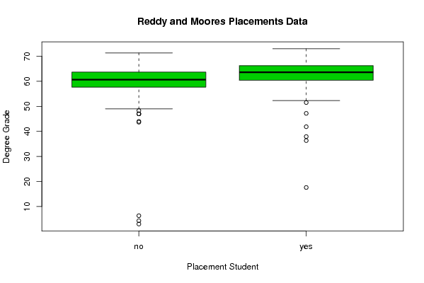
Title produced by software

Boxplot and Trimmed Means

Date of computation

Tue, 19 Oct 2010 11:08:50 +0000

Cite this page as follows

Statistical Computations at FreeStatistics.org, Office for Research Development and Education, URL https://freestatistics.org/blog/index.php?v=date/2010/Oct/19/t1287486540v7cx187fuurxom3.htm/, Retrieved Sun, 28 Apr 2024 21:21:18 +0000

Statistical Computations at FreeStatistics.org, Office for Research Development and Education, URL https://freestatistics.org/blog/index.php?pk=86196, Retrieved Sun, 28 Apr 2024 21:21:18 +0000

QR Codes:

Paste this QR Code to cite your computation.

Original text written by user:

IsPrivate?

No (this computation is public)

User-defined keywords

Estimated Impact

Family? (F = Feedback message, R = changed R code, M = changed R Module, P = changed Parameters, D = changed Data)

-     [Boxplot and Trimmed Means] [Reddy Moores Boxp...] [2010-10-12 16:37:57] [98fd0e87c3eb04e0cc2efde01dbafab6]
- R P   [Boxplot and Trimmed Means] [Reddy-Moores Plac...] [2010-10-13 09:46:26] [98fd0e87c3eb04e0cc2efde01dbafab6]
-    D    [Boxplot and Trimmed Means] [Error with Boxplot] [2010-10-17 09:53:51] [a1af044be13ec2160cfa9b8e01858a75]
- R  D      [Boxplot and Trimmed Means] [Boxplot of Reddy ...] [2010-10-18 08:31:37] [98fd0e87c3eb04e0cc2efde01dbafab6]
-             [Boxplot and Trimmed Means] [Boxplot of Reddy ...] [2010-10-18 08:38:06] [98fd0e87c3eb04e0cc2efde01dbafab6]
- R             [Boxplot and Trimmed Means] [Boxplot of Reddy ...] [2010-10-18 08:42:04] [98fd0e87c3eb04e0cc2efde01dbafab6]
- R               [Boxplot and Trimmed Means] [Reddy Moores Boxp...] [2010-10-18 11:10:52] [98fd0e87c3eb04e0cc2efde01dbafab6]
- R                 [Boxplot and Trimmed Means] [Boxplot 0% trim] [2010-10-18 14:56:34] [98fd0e87c3eb04e0cc2efde01dbafab6]
-                     [Boxplot and Trimmed Means] [20% trim boxplot] [2010-10-18 15:00:15] [98fd0e87c3eb04e0cc2efde01dbafab6]
-                       [Boxplot and Trimmed Means] [20% trim] [2010-10-18 15:13:50] [98fd0e87c3eb04e0cc2efde01dbafab6]
- R P                     [Boxplot and Trimmed Means] [Trim 0%] [2010-10-18 15:18:47] [98fd0e87c3eb04e0cc2efde01dbafab6]
- R  D                      [Boxplot and Trimmed Means] [test] [2010-10-18 16:42:35] [b98453cac15ba1066b407e146608df68]
-   P                         [Boxplot and Trimmed Means] [Reddy-Moores Plac...] [2010-10-18 17:11:37] [98fd0e87c3eb04e0cc2efde01dbafab6]
-    D                            [Boxplot and Trimmed Means] [] [2010-10-19 11:08:50] [888d8c63fc0cbb608262979f3ad7d0e7] [Current]

Feedback Forum

Post a new message

Dataseries X:

Download CSV

Histogram

Boxplots

"no"	3.00
"no"	4.33
"no"	6.33
"no"	43.67
"no"	44.00
"no"	47.00
"no"	47.00
"no"	47.00
"no"	48.33
"no"	49.00
"no"	49.33
"no"	49.67
"no"	51.00
"no"	51.00
"no"	51.00
"no"	51.00
"no"	52.67
"no"	53.33
"no"	53.67
"no"	53.67
"no"	54.00
"no"	54.00
"no"	54.33
"no"	54.33
"no"	54.67
"no"	54.67
"no"	54.67
"no"	55.00
"no"	55.00
"no"	55.33
"no"	55.33
"no"	55.33
"no"	55.67
"no"	55.67
"no"	56.00
"no"	56.00
"no"	56.00
"no"	56.33
"no"	56.33
"no"	56.67
"no"	56.67
"no"	56.67
"no"	56.67
"no"	57.00
"no"	57.33
"no"	57.33
"no"	57.67
"no"	57.67
"no"	58.00
"no"	58.00
"no"	58.00
"no"	58.00
"no"	58.00
"no"	58.00
"no"	58.00
"no"	58.00
"no"	58.33
"no"	58.33
"no"	58.67
"no"	58.67
"no"	58.67
"no"	58.67
"no"	58.67
"no"	58.67
"no"	58.67
"no"	59.00
"no"	59.00
"no"	59.33
"no"	59.33
"no"	59.33
"no"	59.33
"no"	59.33
"no"	59.67
"no"	59.67
"no"	59.67
"no"	59.67
"no"	59.67
"no"	59.67
"no"	60.00
"no"	60.00
"no"	60.00
"no"	60.00
"no"	60.00
"no"	60.00
"no"	60.00
"no"	60.00
"no"	60.00
"no"	60.33
"no"	60.33
"no"	60.33
"no"	60.33
"no"	60.33
"no"	60.33
"no"	60.67
"no"	60.67
"no"	60.67
"no"	60.67
"no"	60.67
"no"	61.00
"no"	61.00
"no"	61.00
"no"	61.00
"no"	61.00
"no"	61.00
"no"	61.33
"no"	61.33
"no"	61.33
"no"	61.33
"no"	61.33
"no"	61.33
"no"	61.33
"no"	61.67
"no"	61.67
"no"	61.67
"no"	61.67
"no"	61.67
"no"	61.67
"no"	61.67
"no"	61.67
"no"	62.00
"no"	62.00
"no"	62.00
"no"	62.00
"no"	62.00
"no"	62.00
"no"	62.33
"no"	62.33
"no"	62.33
"no"	62.33
"no"	62.67
"no"	63.00
"no"	63.00
"no"	63.00
"no"	63.33
"no"	63.33
"no"	63.33
"no"	63.33
"no"	63.33
"no"	63.67
"no"	63.67
"no"	63.67
"no"	63.67
"no"	63.67
"no"	63.67
"no"	63.67
"no"	63.67
"no"	63.67
"no"	64.00
"no"	64.00
"no"	64.00
"no"	64.00
"no"	64.00
"no"	64.00
"no"	64.00
"no"	64.00
"no"	64.33
"no"	64.33
"no"	64.67
"no"	64.67
"no"	64.67
"no"	64.67
"no"	65.00
"no"	65.00
"no"	65.00
"no"	65.33
"no"	65.33
"no"	65.67
"no"	65.67
"no"	65.67
"no"	65.67
"no"	65.67
"no"	66.00
"no"	66.00
"no"	66.00
"no"	66.00
"no"	66.33
"no"	66.33
"no"	66.67
"no"	66.67
"no"	66.67
"no"	66.67
"no"	67.33
"no"	67.67
"no"	68.00
"no"	68.67
"no"	69.00
"no"	70.00
"no"	70.33
"no"	71.33
"yes"	17.60
"yes"	36.33
"yes"	37.93
"yes"	41.87
"yes"	47.20
"yes"	51.53
"yes"	52.33
"yes"	52.67
"yes"	53.87
"yes"	54.20
"yes"	54.73
"yes"	55.00
"yes"	55.07
"yes"	55.47
"yes"	55.93
"yes"	56.20
"yes"	56.33
"yes"	56.67
"yes"	57.13
"yes"	57.47
"yes"	57.47
"yes"	57.67
"yes"	57.67
"yes"	57.80
"yes"	57.87
"yes"	58.07
"yes"	58.20
"yes"	58.27
"yes"	58.27
"yes"	58.33
"yes"	58.40
"yes"	58.80
"yes"	58.80
"yes"	58.93
"yes"	59.00
"yes"	59.13
"yes"	59.13
"yes"	59.40
"yes"	59.47
"yes"	59.53
"yes"	59.53
"yes"	59.53
"yes"	59.60
"yes"	59.67
"yes"	59.67
"yes"	59.73
"yes"	59.73
"yes"	59.73
"yes"	59.80
"yes"	59.80
"yes"	59.87
"yes"	60.13
"yes"	60.13
"yes"	60.13
"yes"	60.33
"yes"	60.40
"yes"	60.47
"yes"	60.73
"yes"	60.80
"yes"	60.87
"yes"	61.00
"yes"	61.00
"yes"	61.27
"yes"	61.27
"yes"	61.33
"yes"	61.40
"yes"	61.40
"yes"	61.47
"yes"	61.47
"yes"	61.60
"yes"	61.60
"yes"	61.60
"yes"	61.67
"yes"	61.80
"yes"	61.87
"yes"	61.93
"yes"	61.93
"yes"	61.93
"yes"	62.00
"yes"	62.13
"yes"	62.20
"yes"	62.40
"yes"	62.40
"yes"	62.40
"yes"	62.40
"yes"	62.40
"yes"	62.53
"yes"	62.60
"yes"	62.60
"yes"	62.60
"yes"	62.60
"yes"	62.67
"yes"	62.67
"yes"	62.80
"yes"	62.80
"yes"	62.80
"yes"	62.87
"yes"	62.87
"yes"	62.93
"yes"	62.93
"yes"	63.00
"yes"	63.00
"yes"	63.07
"yes"	63.13
"yes"	63.20
"yes"	63.27
"yes"	63.33
"yes"	63.33
"yes"	63.47
"yes"	63.53
"yes"	63.53
"yes"	63.53
"yes"	63.60
"yes"	63.67
"yes"	63.67
"yes"	63.67
"yes"	63.73
"yes"	63.73
"yes"	63.73
"yes"	63.87
"yes"	64.00
"yes"	64.07
"yes"	64.07
"yes"	64.07
"yes"	64.13
"yes"	64.20
"yes"	64.20
"yes"	64.27
"yes"	64.27
"yes"	64.40
"yes"	64.47
"yes"	64.60
"yes"	64.60
"yes"	64.67
"yes"	64.67
"yes"	64.67
"yes"	64.67
"yes"	64.67
"yes"	64.67
"yes"	64.67
"yes"	64.67
"yes"	64.73
"yes"	64.80
"yes"	64.87
"yes"	65.00
"yes"	65.00
"yes"	65.07
"yes"	65.07
"yes"	65.20
"yes"	65.47
"yes"	65.47
"yes"	65.60
"yes"	65.67
"yes"	65.67
"yes"	65.80
"yes"	65.80
"yes"	65.80
"yes"	65.93
"yes"	66.00
"yes"	66.00
"yes"	66.00
"yes"	66.00
"yes"	66.00
"yes"	66.00
"yes"	66.00
"yes"	66.07
"yes"	66.20
"yes"	66.20
"yes"	66.27
"yes"	66.27
"yes"	66.47
"yes"	66.53
"yes"	66.53
"yes"	66.53
"yes"	66.60
"yes"	66.73
"yes"	66.73
"yes"	66.73
"yes"	66.73
"yes"	66.80
"yes"	66.87
"yes"	66.93
"yes"	67.07
"yes"	67.13
"yes"	67.33
"yes"	67.47
"yes"	67.47
"yes"	67.53
"yes"	67.60
"yes"	67.60
"yes"	67.80
"yes"	68.07
"yes"	68.60
"yes"	68.67
"yes"	68.67
"yes"	68.73
"yes"	68.80
"yes"	68.80
"yes"	68.87
"yes"	69.53
"yes"	69.60
"yes"	69.60
"yes"	69.87
"yes"	69.93
"yes"	70.07
"yes"	70.07
"yes"	70.47
"yes"	70.67
"yes"	70.67
"yes"	70.73
"yes"	70.73
"yes"	70.73
"yes"	70.73
"yes"	70.80
"yes"	70.80
"yes"	71.07
"yes"	71.47
"yes"	71.53
"yes"	71.67
"yes"	71.67
"yes"	72.07
"yes"	72.73
"yes"	72.73
"yes"	72.87
"yes"	73.00

Summary of computational transaction
Raw Input	view raw input (R code)
Raw Output	view raw output of R engine
Computing time	2 seconds
R Server	'RServer@AstonUniversity' @ vre.aston.ac.uk

\begin{tabular}{lllllllll}
\hline
Summary of computational transaction \tabularnewline
Raw Input & view raw input (R code)  \tabularnewline
Raw Output & view raw output of R engine  \tabularnewline
Computing time & 2 seconds \tabularnewline
R Server & 'RServer@AstonUniversity' @ vre.aston.ac.uk \tabularnewline
\hline
\end{tabular}
%Source: https://freestatistics.org/blog/index.php?pk=86196&T=0

[TABLE]
[ROW][C]Summary of computational transaction[/C][/ROW]
[ROW][C]Raw Input[/C][C]view raw input (R code) [/C][/ROW]
[ROW][C]Raw Output[/C][C]view raw output of R engine [/C][/ROW]
[ROW][C]Computing time[/C][C]2 seconds[/C][/ROW]
[ROW][C]R Server[/C][C]'RServer@AstonUniversity' @ vre.aston.ac.uk[/C][/ROW]
[/TABLE]
Source: https://freestatistics.org/blog/index.php?pk=86196&T=0

Globally Unique Identifier (entire table): ba.freestatistics.org/blog/index.php?pk=86196&T=0

As an alternative you can also use a QR Code:

The GUIDs for individual cells are displayed in the table below:

Summary of computational transaction
Raw Input	view raw input (R code)
Raw Output	view raw output of R engine
Computing time	2 seconds
R Server	'RServer@AstonUniversity' @ vre.aston.ac.uk

Boxplot statistics
Placement	lower whisker	lower hinge	median	upper hinge	upper whisker
no	49	57.67	60.67	63.67	71.33
yes	52.33	60.47	63.6	66.27	73

\begin{tabular}{lllllllll}
\hline
Boxplot statistics \tabularnewline
Placement & lower whisker & lower hinge & median & upper hinge & upper whisker \tabularnewline
no & 49 & 57.67 & 60.67 & 63.67 & 71.33 \tabularnewline
yes & 52.33 & 60.47 & 63.6 & 66.27 & 73 \tabularnewline
\hline
\end{tabular}
%Source: https://freestatistics.org/blog/index.php?pk=86196&T=1

[TABLE]
[ROW][C]Boxplot statistics[/C][/ROW]
[ROW][C]Placement[/C][C]lower whisker[/C][C]lower hinge[/C][C]median[/C][C]upper hinge[/C][C]upper whisker[/C][/ROW]
[ROW][C]no[/C][C]49[/C][C]57.67[/C][C]60.67[/C][C]63.67[/C][C]71.33[/C][/ROW]
[ROW][C]yes[/C][C]52.33[/C][C]60.47[/C][C]63.6[/C][C]66.27[/C][C]73[/C][/ROW]
[/TABLE]
Source: https://freestatistics.org/blog/index.php?pk=86196&T=1

Globally Unique Identifier (entire table): ba.freestatistics.org/blog/index.php?pk=86196&T=1

As an alternative you can also use a QR Code:

The GUIDs for individual cells are displayed in the table below:

Boxplot statistics
Placement	lower whisker	lower hinge	median	upper hinge	upper whisker
no	49	57.67	60.67	63.67	71.33
yes	52.33	60.47	63.6	66.27	73

Trimmed Mean Equation
No Placement	Placement
59.3018518518519	63.0598222222222

\begin{tabular}{lllllllll}
\hline
Trimmed Mean Equation \tabularnewline
No Placement & Placement \tabularnewline
59.3018518518519 & 63.0598222222222 \tabularnewline
\hline
\end{tabular}
%Source: https://freestatistics.org/blog/index.php?pk=86196&T=2

[TABLE]
[ROW][C]Trimmed Mean Equation[/C][/ROW]
[ROW][C]No Placement[/C][C]Placement[/C][/ROW]
[ROW][C]59.3018518518519[/C][C]63.0598222222222[/C][/ROW]
[/TABLE]
Source: https://freestatistics.org/blog/index.php?pk=86196&T=2

Globally Unique Identifier (entire table): ba.freestatistics.org/blog/index.php?pk=86196&T=2

As an alternative you can also use a QR Code:

The GUIDs for individual cells are displayed in the table below:

Trimmed Mean Equation
No Placement	Placement
59.3018518518519	63.0598222222222

Figure 1

PNG link

Postscript link

PDF link

Parameters (Session):

par1 = 3 ; par2 = FALSE ; par3 = 0 ; par4 = 1 ; par5 = 2 ;

Parameters (R input):

par1 = 3 ; par2 = FALSE ; par3 = 0 ; par4 = 1 ; par5 = 2 ;

R code (references can be found in the software module):

par1 <- as.numeric(par1) # colour
par2<- as.logical(par2) # notches
par3<-as.numeric(par3) # percentage trim
if(par3>45){par3<-45;warning('trim limited to 45%')}
if(par3<0){par3<-0;warning('negative trim makes no sense. Trim is zero.')}
par4 <- as.numeric(par4) #factor column
par5 <- as.numeric(par5) # response column
x <- t(x)
x1<-as.numeric(x[,par5]) # response
f1<-as.character(x[,par4]) # factor
x2<-x1[f1=='no']
f2 <- f1[f1=='no']
lotrm<-as.integer(length(x2)*par3/100)
hitrm<-as.integer(length(x2)*(100-par3)/100)
srt<-order(x2,f2)
trmx1<-x2[srt[lotrm:hitrm]]
trmf1<-f2[srt[lotrm:hitrm]]
x3<-x1[f1=='yes']
f3 <- f1[f1=='yes']
lotrm<-as.integer(length(x3)*par3/100)
hitrm<-as.integer(length(x3)*(100-par3)/100)
srt<-order(x3,f3)
trmx2<-x3[srt[lotrm:hitrm]]
trmf2<-f3[srt[lotrm:hitrm]]
xtrm<-c(trmx1,trmx2)
ftrm<-c(trmf1,trmf2)
xtrm[1:6]
ftrm[1:6]
bitmap(file='test1.png')
r<-boxplot(xtrm~as.factor(ftrm), col=par1, notch=par2, main='Reddy and Moores Placements Data', xlab='Placement Student', ylab='Degree Grade')
dev.off()
load(file='createtable')
a<-table.start()
a<-table.row.start(a)
a<-table.element(a,hyperlink('overview.htm','Boxplot statistics','Boxplot overview'),6,TRUE)
a<-table.row.end(a)
a<-table.row.start(a)
a<-table.element(a,'Placement',1,TRUE)
a<-table.element(a,hyperlink('lower_whisker.htm','lower whisker','definition of lower whisker'),1,TRUE)
a<-table.element(a,hyperlink('lower_hinge.htm','lower hinge','definition of lower hinge'),1,TRUE)
a<-table.element(a,hyperlink('central_tendency.htm','median','definitions about measures of central tendency'),1,TRUE)
a<-table.element(a,hyperlink('upper_hinge.htm','upper hinge','definition of upper hinge'),1,TRUE)
a<-table.element(a,hyperlink('upper_whisker.htm','upper whisker','definition of upper whisker'),1,TRUE)
a<-table.row.end(a)
a<-table.row.start(a)
a<-table.element(a,'no',1,TRUE)
for (j in 1:5)
{
a<-table.element(a,r$stats[j,1])
}
a<-table.row.end(a)
a<-table.row.start(a)
a<-table.element(a,'yes',1,TRUE)
for (j in 1:5)
{
a<-table.element(a,r$stats[j,2])
}
a<-table.row.end(a)
a<-table.end(a)
table.save(a,file='mytable.tab')
tr.mns<-tapply(x1,f1,mean, trim=par3/100)
a<-table.start()
a<-table.row.start(a)
a<-table.element(a,hyperlink('trimmed_mean.htm','Trimmed Mean Equation','Trimmed Mean'),2,TRUE)
a<-table.row.end(a)
a<-table.row.start(a)
a<-table.element(a,'No Placement')
a<-table.element(a,'Placement')
a<-table.row.end(a)
a<-table.row.start(a)
a<-table.element(a,tr.mns[1])
a<-table.element(a,tr.mns[2])
a<-table.row.end(a)
a<-table.end(a)
table.save(a,file='mytable1.tab')

Free Statistics

Description of Statistical Computation

Tree of Dependent Computations

Dataset

Tables (Output of Computation)

Figures (Output of Computation)

Input Parameters & R Code