Free Statistics
of Irreproducible Research!
Description of Statistical Computation | |||||||||||||||||||||||||||||||||||||||||||||||||||||||||||||||||
|---|---|---|---|---|---|---|---|---|---|---|---|---|---|---|---|---|---|---|---|---|---|---|---|---|---|---|---|---|---|---|---|---|---|---|---|---|---|---|---|---|---|---|---|---|---|---|---|---|---|---|---|---|---|---|---|---|---|---|---|---|---|---|---|---|---|
| Author's title | |||||||||||||||||||||||||||||||||||||||||||||||||||||||||||||||||
| Author | *The author of this computation has been verified* | ||||||||||||||||||||||||||||||||||||||||||||||||||||||||||||||||
| R Software Module | rwasp_edabi.wasp | ||||||||||||||||||||||||||||||||||||||||||||||||||||||||||||||||
| Title produced by software | Bivariate Explorative Data Analysis | ||||||||||||||||||||||||||||||||||||||||||||||||||||||||||||||||
| Date of computation | Thu, 29 Oct 2009 09:06:05 -0600 | ||||||||||||||||||||||||||||||||||||||||||||||||||||||||||||||||
| Cite this page as follows | Statistical Computations at FreeStatistics.org, Office for Research Development and Education, URL https://freestatistics.org/blog/index.php?v=date/2009/Oct/29/t125682887487jusgyb8mrqpxz.htm/, Retrieved Mon, 29 Apr 2024 07:54:49 +0000 | ||||||||||||||||||||||||||||||||||||||||||||||||||||||||||||||||
| Statistical Computations at FreeStatistics.org, Office for Research Development and Education, URL https://freestatistics.org/blog/index.php?pk=52008, Retrieved Mon, 29 Apr 2024 07:54:49 +0000 | |||||||||||||||||||||||||||||||||||||||||||||||||||||||||||||||||
| QR Codes: | |||||||||||||||||||||||||||||||||||||||||||||||||||||||||||||||||
|
| |||||||||||||||||||||||||||||||||||||||||||||||||||||||||||||||||
| Original text written by user: | |||||||||||||||||||||||||||||||||||||||||||||||||||||||||||||||||
| IsPrivate? | No (this computation is public) | ||||||||||||||||||||||||||||||||||||||||||||||||||||||||||||||||
| User-defined keywords | |||||||||||||||||||||||||||||||||||||||||||||||||||||||||||||||||
| Estimated Impact | 154 | ||||||||||||||||||||||||||||||||||||||||||||||||||||||||||||||||
Tree of Dependent Computations | |||||||||||||||||||||||||||||||||||||||||||||||||||||||||||||||||
| Family? (F = Feedback message, R = changed R code, M = changed R Module, P = changed Parameters, D = changed Data) | |||||||||||||||||||||||||||||||||||||||||||||||||||||||||||||||||
| F [Trivariate Scatterplots] [trivariate analysis] [2008-11-13 08:14:40] [3b5d63cebdc58ed6c519cdb5b6a36d46] - RMPD [Bivariate Explorative Data Analysis] [(Y[t] - g - h Z[t...] [2009-10-28 12:27:46] [74be16979710d4c4e7c6647856088456] - D [Bivariate Explorative Data Analysis] [WS5 (Y[t] - g - h...] [2009-10-29 15:06:05] [37de18e38c1490dd77c2b362ed87f3bb] [Current] - M [Bivariate Explorative Data Analysis] [BDM 4] [2009-11-03 11:56:09] [f5d341d4bbba73282fc6e80153a6d315] - M [Bivariate Explorative Data Analysis] [TG4] [2009-11-03 12:03:41] [a21bac9c8d3d56fdec8be4e719e2c7ed] - M [Bivariate Explorative Data Analysis] [P7] [2009-12-15 09:49:30] [f5d341d4bbba73282fc6e80153a6d315] | |||||||||||||||||||||||||||||||||||||||||||||||||||||||||||||||||
| Feedback Forum | |||||||||||||||||||||||||||||||||||||||||||||||||||||||||||||||||
Post a new message | |||||||||||||||||||||||||||||||||||||||||||||||||||||||||||||||||
Dataset | |||||||||||||||||||||||||||||||||||||||||||||||||||||||||||||||||
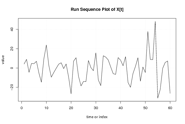
| Dataseries X: | |||||||||||||||||||||||||||||||||||||||||||||||||||||||||||||||||
4.120575483 8.926511718 -4.46024537 4.727882162 4.432447952 6.950256655 -5.32280306 -14.69266743 9.590894311 23.81920504 2.589069408 -9.504994357 -4.66481116 -0.229193754 4.008248556 5.383133174 -0.630564198 4.148431753 -9.51138505 -26.78764011 7.089985394 10.64478195 -8.66297919 -18.5246209 -13.93557738 -14.03466139 7.721960062 0.405521803 -2.811832441 15.73565743 -12.38854196 -18.25109965 12.66670905 11.26625459 8.322876048 1.079497504 -5.869817274 -6.599952905 10.76077988 8.019226242 2.303242442 11.71054912 -15.01182537 -19.98990534 -5.734654326 1.602333524 10.6078153 -13.65884666 0.998690786 -4.683954969 37.83385373 8.819708971 8.615611775 48.25943771 -31.23279409 -22.29124044 -0.374802185 5.6841057 7.232050034 -26.2158943 | |||||||||||||||||||||||||||||||||||||||||||||||||||||||||||||||||
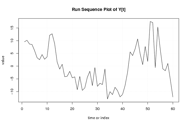
| Dataseries Y: | |||||||||||||||||||||||||||||||||||||||||||||||||||||||||||||||||
9.566151798 10.1585264 8.675824146 8.49107495 6.150900994 3.328024789 2.524800673 4.548854048 2.704278807 3.633603244 12.10954987 12.70192447 8.815998101 1.57024569 -1.180777783 0.717175271 -4.162302863 -3.966704149 -2.052630515 -4.583132122 -4.220081962 -9.256162024 -4.04326556 -9.523920864 -8.538301891 -4.367933722 -2.009284847 -7.653860088 -0.568803499 -7.929806713 -6.76148549 -7.212508963 -1.135385169 -12.89756555 -10.03891668 -11.1802678 -8.313993526 -9.638046901 -12.08175237 -11.12837455 -7.61076941 -2.385846259 5.577203902 4.151973357 6.778073679 10.66486982 4.795064035 0.592402302 7.721419347 1.836362757 17.51348655 17.11783543 -0.587795425 15.36972868 6.50283962 -1.050538193 -1.805962952 1.055602646 -5.343220184 -12.14439735 | |||||||||||||||||||||||||||||||||||||||||||||||||||||||||||||||||
Tables (Output of Computation) | |||||||||||||||||||||||||||||||||||||||||||||||||||||||||||||||||
| |||||||||||||||||||||||||||||||||||||||||||||||||||||||||||||||||
Figures (Output of Computation) | |||||||||||||||||||||||||||||||||||||||||||||||||||||||||||||||||
Input Parameters & R Code | |||||||||||||||||||||||||||||||||||||||||||||||||||||||||||||||||
| Parameters (Session): | |||||||||||||||||||||||||||||||||||||||||||||||||||||||||||||||||
| par1 = 0 ; par2 = 36 ; | |||||||||||||||||||||||||||||||||||||||||||||||||||||||||||||||||
| Parameters (R input): | |||||||||||||||||||||||||||||||||||||||||||||||||||||||||||||||||
| par1 = 0 ; par2 = 36 ; | |||||||||||||||||||||||||||||||||||||||||||||||||||||||||||||||||
| R code (references can be found in the software module): | |||||||||||||||||||||||||||||||||||||||||||||||||||||||||||||||||
par1 <- as.numeric(par1) | |||||||||||||||||||||||||||||||||||||||||||||||||||||||||||||||||