Free Statistics
of Irreproducible Research!
Description of Statistical Computation | |||||||||||||||||||||||||||||||||||||||||
|---|---|---|---|---|---|---|---|---|---|---|---|---|---|---|---|---|---|---|---|---|---|---|---|---|---|---|---|---|---|---|---|---|---|---|---|---|---|---|---|---|---|
| Author's title | |||||||||||||||||||||||||||||||||||||||||
| Author | *The author of this computation has been verified* | ||||||||||||||||||||||||||||||||||||||||
| R Software Module | rwasp_cloud.wasp | ||||||||||||||||||||||||||||||||||||||||
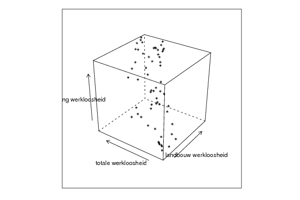
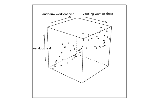
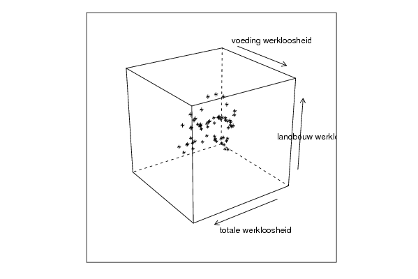
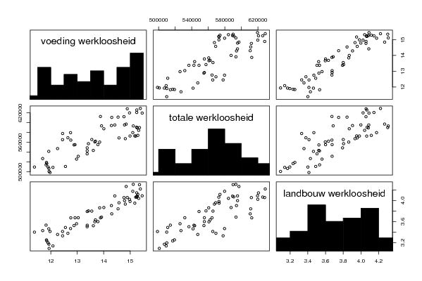
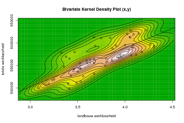
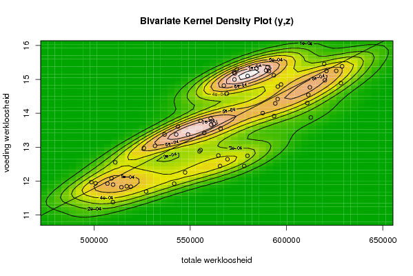
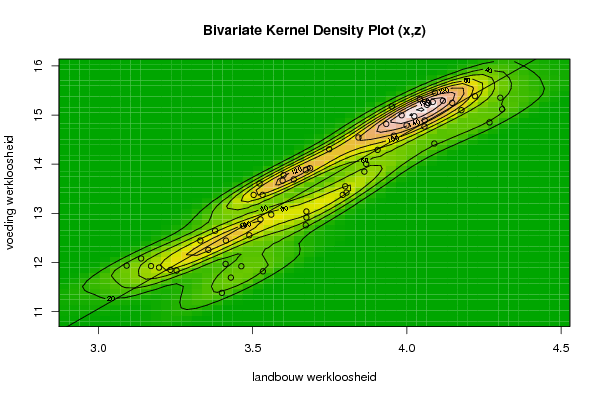
| Title produced by software | Trivariate Scatterplots | ||||||||||||||||||||||||||||||||||||||||
| Date of computation | Thu, 13 Nov 2008 01:14:40 -0700 | ||||||||||||||||||||||||||||||||||||||||
| Cite this page as follows | Statistical Computations at FreeStatistics.org, Office for Research Development and Education, URL https://freestatistics.org/blog/index.php?v=date/2008/Nov/13/t1226564141mjuberuockx7m4i.htm/, Retrieved Wed, 20 May 2026 10:50:17 +0000 | ||||||||||||||||||||||||||||||||||||||||
| Statistical Computations at FreeStatistics.org, Office for Research Development and Education, URL https://freestatistics.org/blog/index.php?pk=24476, Retrieved Wed, 20 May 2026 10:50:17 +0000 | |||||||||||||||||||||||||||||||||||||||||
| QR Codes: | |||||||||||||||||||||||||||||||||||||||||
|
| |||||||||||||||||||||||||||||||||||||||||
| Original text written by user: | |||||||||||||||||||||||||||||||||||||||||
| IsPrivate? | No (this computation is public) | ||||||||||||||||||||||||||||||||||||||||
| User-defined keywords | natalie en evelyn | ||||||||||||||||||||||||||||||||||||||||
| Estimated Impact | 643 | ||||||||||||||||||||||||||||||||||||||||
Tree of Dependent Computations | |||||||||||||||||||||||||||||||||||||||||
| Family? (F = Feedback message, R = changed R code, M = changed R Module, P = changed Parameters, D = changed Data) | |||||||||||||||||||||||||||||||||||||||||
| F [Trivariate Scatterplots] [trivariate analysis] [2008-11-13 08:14:40] [32a7b12f2bdf14b45f7a9a96ba1ab98d] [Current] - PD [Trivariate Scatterplots] [college] [2009-10-28 12:04:53] [74be16979710d4c4e7c6647856088456] - RMPD [Partial Correlation] [college] [2009-10-28 12:07:04] [74be16979710d4c4e7c6647856088456] - RMPD [Bivariate Explorative Data Analysis] [college] [2009-10-28 12:09:10] [74be16979710d4c4e7c6647856088456] - RMPD [Bivariate Explorative Data Analysis] [college Y=f(Z)] [2009-10-28 12:19:32] [74be16979710d4c4e7c6647856088456] - D [Bivariate Explorative Data Analysis] [WS5 berekening Y=...] [2009-10-29 14:37:50] [42ad1186d39724f834063794eac7cea3] - M [Bivariate Explorative Data Analysis] [BDM2] [2009-11-03 11:53:00] [f5d341d4bbba73282fc6e80153a6d315] - M [Bivariate Explorative Data Analysis] [TG2] [2009-11-03 11:59:56] [a21bac9c8d3d56fdec8be4e719e2c7ed] - M [Bivariate Explorative Data Analysis] [P5] [2009-12-15 09:47:24] [f5d341d4bbba73282fc6e80153a6d315] - RMPD [Bivariate Explorative Data Analysis] [college X=f(Z)] [2009-10-28 12:22:29] [74be16979710d4c4e7c6647856088456] - D [Bivariate Explorative Data Analysis] [WS5 X=f(Z)] [2009-10-29 14:46:05] [42ad1186d39724f834063794eac7cea3] - M [Bivariate Explorative Data Analysis] [BDM3] [2009-11-03 11:54:58] [f5d341d4bbba73282fc6e80153a6d315] - M [Bivariate Explorative Data Analysis] [TG3] [2009-11-03 12:01:14] [a21bac9c8d3d56fdec8be4e719e2c7ed] - M [Bivariate Explorative Data Analysis] [P6] [2009-12-15 09:48:17] [f5d341d4bbba73282fc6e80153a6d315] - RMPD [Bivariate Explorative Data Analysis] [(Y[t] - g - h Z[t...] [2009-10-28 12:27:46] [74be16979710d4c4e7c6647856088456] - D [Bivariate Explorative Data Analysis] [WS5 (Y[t] - g - h...] [2009-10-29 15:06:05] [42ad1186d39724f834063794eac7cea3] - M [Bivariate Explorative Data Analysis] [BDM 4] [2009-11-03 11:56:09] [f5d341d4bbba73282fc6e80153a6d315] - M [Bivariate Explorative Data Analysis] [TG4] [2009-11-03 12:03:41] [a21bac9c8d3d56fdec8be4e719e2c7ed] - M [Bivariate Explorative Data Analysis] [P7] [2009-12-15 09:49:30] [f5d341d4bbba73282fc6e80153a6d315] | |||||||||||||||||||||||||||||||||||||||||
| Feedback Forum | |||||||||||||||||||||||||||||||||||||||||
Post a new message | |||||||||||||||||||||||||||||||||||||||||
Dataset | |||||||||||||||||||||||||||||||||||||||||
| Dataseries X: | |||||||||||||||||||||||||||||||||||||||||
3.253 3.233 3.196 3.138 3.091 3.17 3.378 3.468 3.33 3.413 3.356 3.525 3.633 3.597 3.6 3.522 3.503 3.532 3.686 3.748 3.672 3.843 3.905 3.999 4.07 4.084 4.042 3.951 3.933 3.958 4.147 4.221 4.058 4.057 4.089 4.268 4.309 4.303 4.177 4.117 4.065 3.983 4.091 4.067 4.024 3.868 3.8 3.804 3.862 3.792 3.674 3.56 3.489 3.412 3.674 3.672 3.463 3.429 3.4 3.533 | |||||||||||||||||||||||||||||||||||||||||
| Dataseries Y: | |||||||||||||||||||||||||||||||||||||||||
519164 517009 509933 509127 500857 506971 569323 579714 577992 565464 547344 554788 562325 560854 555332 543599 536662 542722 593530 610763 612613 611324 594167 595454 590865 589379 584428 573100 567456 569028 620735 628884 628232 612117 595404 597141 593408 590072 579799 574205 572775 572942 619567 625809 619916 587625 565742 557274 560576 548854 531673 525919 511038 498662 555362 564591 541657 527070 509846 514258 | |||||||||||||||||||||||||||||||||||||||||
| Dataseries Z: | |||||||||||||||||||||||||||||||||||||||||
11.836 11.85 11.897 12.082 11.936 11.928 12.646 12.747 12.447 12.445 12.257 12.878 13.69 13.665 13.78 13.608 13.375 13.376 13.918 14.304 13.877 14.543 14.291 14.788 15.241 15.265 15.322 15.175 14.817 14.579 15.247 15.385 14.891 14.766 14.42 14.85 15.117 15.352 15.099 15.291 15.208 14.995 15.454 15.251 14.975 14.005 13.55 13.422 13.848 13.376 13.038 12.974 12.554 11.971 12.916 12.757 11.924 11.693 11.382 11.821 | |||||||||||||||||||||||||||||||||||||||||
Tables (Output of Computation) | |||||||||||||||||||||||||||||||||||||||||
| |||||||||||||||||||||||||||||||||||||||||
Figures (Output of Computation) | |||||||||||||||||||||||||||||||||||||||||
Input Parameters & R Code | |||||||||||||||||||||||||||||||||||||||||
| Parameters (Session): | |||||||||||||||||||||||||||||||||||||||||
| par1 = 50 ; par2 = 50 ; par3 = Y ; par4 = Y ; par5 = landbouw werkloosheid ; par6 = totale werkloosheid ; par7 = voeding werkloosheid ; | |||||||||||||||||||||||||||||||||||||||||
| Parameters (R input): | |||||||||||||||||||||||||||||||||||||||||
| par1 = 50 ; par2 = 50 ; par3 = Y ; par4 = Y ; par5 = landbouw werkloosheid ; par6 = totale werkloosheid ; par7 = voeding werkloosheid ; | |||||||||||||||||||||||||||||||||||||||||
| R code (references can be found in the software module): | |||||||||||||||||||||||||||||||||||||||||
x <- array(x,dim=c(length(x),1)) | |||||||||||||||||||||||||||||||||||||||||