Free Statistics
of Irreproducible Research!
Description of Statistical Computation | |||||||||||||||||||||||||||||||||||||||||||||||||||||||||||||||||
|---|---|---|---|---|---|---|---|---|---|---|---|---|---|---|---|---|---|---|---|---|---|---|---|---|---|---|---|---|---|---|---|---|---|---|---|---|---|---|---|---|---|---|---|---|---|---|---|---|---|---|---|---|---|---|---|---|---|---|---|---|---|---|---|---|---|
| Author's title | |||||||||||||||||||||||||||||||||||||||||||||||||||||||||||||||||
| Author | *The author of this computation has been verified* | ||||||||||||||||||||||||||||||||||||||||||||||||||||||||||||||||
| R Software Module | rwasp_edabi.wasp | ||||||||||||||||||||||||||||||||||||||||||||||||||||||||||||||||
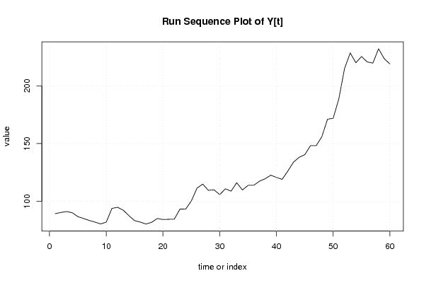
| Title produced by software | Bivariate Explorative Data Analysis | ||||||||||||||||||||||||||||||||||||||||||||||||||||||||||||||||
| Date of computation | Thu, 29 Oct 2009 08:37:50 -0600 | ||||||||||||||||||||||||||||||||||||||||||||||||||||||||||||||||
| Cite this page as follows | Statistical Computations at FreeStatistics.org, Office for Research Development and Education, URL https://freestatistics.org/blog/index.php?v=date/2009/Oct/29/t12568271484xg6ldrxhtufj2l.htm/, Retrieved Mon, 30 Jun 2025 21:42:46 +0000 | ||||||||||||||||||||||||||||||||||||||||||||||||||||||||||||||||
| Statistical Computations at FreeStatistics.org, Office for Research Development and Education, URL https://freestatistics.org/blog/index.php?pk=51999, Retrieved Mon, 30 Jun 2025 21:42:46 +0000 | |||||||||||||||||||||||||||||||||||||||||||||||||||||||||||||||||
| QR Codes: | |||||||||||||||||||||||||||||||||||||||||||||||||||||||||||||||||
|
| |||||||||||||||||||||||||||||||||||||||||||||||||||||||||||||||||
| Original text written by user: | |||||||||||||||||||||||||||||||||||||||||||||||||||||||||||||||||
| IsPrivate? | No (this computation is public) | ||||||||||||||||||||||||||||||||||||||||||||||||||||||||||||||||
| User-defined keywords | |||||||||||||||||||||||||||||||||||||||||||||||||||||||||||||||||
| Estimated Impact | 275 | ||||||||||||||||||||||||||||||||||||||||||||||||||||||||||||||||
Tree of Dependent Computations | |||||||||||||||||||||||||||||||||||||||||||||||||||||||||||||||||
| Family? (F = Feedback message, R = changed R code, M = changed R Module, P = changed Parameters, D = changed Data) | |||||||||||||||||||||||||||||||||||||||||||||||||||||||||||||||||
| F [Trivariate Scatterplots] [trivariate analysis] [2008-11-13 08:14:40] [3b5d63cebdc58ed6c519cdb5b6a36d46] - RMPD [Bivariate Explorative Data Analysis] [college Y=f(Z)] [2009-10-28 12:19:32] [74be16979710d4c4e7c6647856088456] - D [Bivariate Explorative Data Analysis] [WS5 berekening Y=...] [2009-10-29 14:37:50] [37de18e38c1490dd77c2b362ed87f3bb] [Current] - M [Bivariate Explorative Data Analysis] [BDM2] [2009-11-03 11:53:00] [f5d341d4bbba73282fc6e80153a6d315] - M [Bivariate Explorative Data Analysis] [TG2] [2009-11-03 11:59:56] [a21bac9c8d3d56fdec8be4e719e2c7ed] - M [Bivariate Explorative Data Analysis] [P5] [2009-12-15 09:47:24] [f5d341d4bbba73282fc6e80153a6d315] | |||||||||||||||||||||||||||||||||||||||||||||||||||||||||||||||||
| Feedback Forum | |||||||||||||||||||||||||||||||||||||||||||||||||||||||||||||||||
Post a new message | |||||||||||||||||||||||||||||||||||||||||||||||||||||||||||||||||
Dataset | |||||||||||||||||||||||||||||||||||||||||||||||||||||||||||||||||
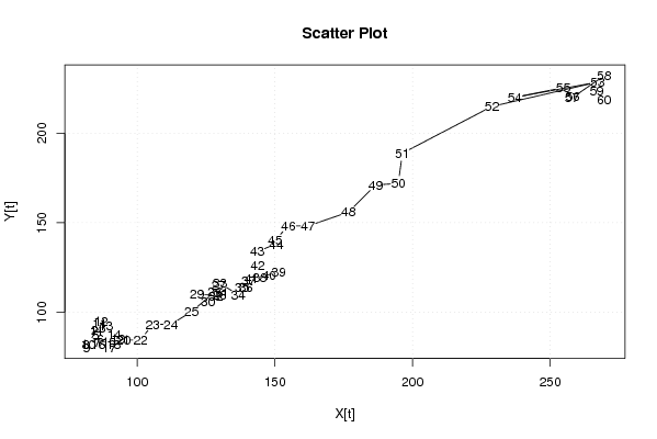
| Dataseries X: | |||||||||||||||||||||||||||||||||||||||||||||||||||||||||||||||||
84 84.5 87.3 86.3 85 86.5 85.4 81.2 81.5 82.2 86.4 86.9 88.6 91.6 89.7 85.9 89.8 91.4 93.1 95.1 94.9 101.2 105.6 112.2 119.7 128.2 129.6 129.9 121.7 125.7 130.4 128.5 130 136.7 138.1 139.5 140.4 144.6 151.4 147.9 141.5 143.8 143.6 150.5 150.1 154.9 162.1 176.7 186.6 194.8 196.3 228.8 267.2 237.2 254.7 258.2 257.9 269.6 266.9 269.6 | |||||||||||||||||||||||||||||||||||||||||||||||||||||||||||||||||
| Dataseries Y: | |||||||||||||||||||||||||||||||||||||||||||||||||||||||||||||||||
89.3 90.3 91.1 90.1 86.7 85.1 83.4 82 80.4 81.9 93.8 94.8 92.3 87.5 83.2 82 80.3 81.8 85.1 84.2 84.4 84.5 93.3 93.2 100.3 111.4 114.9 109.5 109.9 105.8 110.8 108.8 116.1 109.8 113.8 113.8 117.4 119.5 122.6 120.7 119 126.1 133.9 138.1 140.4 148.2 148.2 155.9 171.1 171.9 188.8 214.9 228.5 220 225.4 220.7 219.7 232.1 223.5 218.9 | |||||||||||||||||||||||||||||||||||||||||||||||||||||||||||||||||
Tables (Output of Computation) | |||||||||||||||||||||||||||||||||||||||||||||||||||||||||||||||||
| |||||||||||||||||||||||||||||||||||||||||||||||||||||||||||||||||
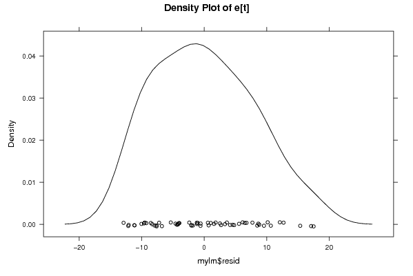
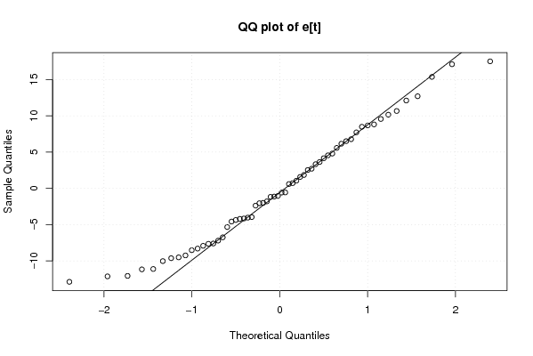
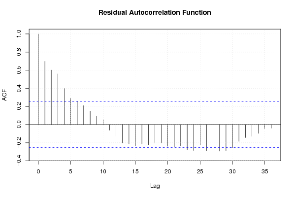
Figures (Output of Computation) | |||||||||||||||||||||||||||||||||||||||||||||||||||||||||||||||||
Input Parameters & R Code | |||||||||||||||||||||||||||||||||||||||||||||||||||||||||||||||||
| Parameters (Session): | |||||||||||||||||||||||||||||||||||||||||||||||||||||||||||||||||
| par1 = 0 ; par2 = 36 ; | |||||||||||||||||||||||||||||||||||||||||||||||||||||||||||||||||
| Parameters (R input): | |||||||||||||||||||||||||||||||||||||||||||||||||||||||||||||||||
| par1 = 0 ; par2 = 36 ; | |||||||||||||||||||||||||||||||||||||||||||||||||||||||||||||||||
| R code (references can be found in the software module): | |||||||||||||||||||||||||||||||||||||||||||||||||||||||||||||||||
par1 <- as.numeric(par1) | |||||||||||||||||||||||||||||||||||||||||||||||||||||||||||||||||