Free Statistics
of Irreproducible Research!
Description of Statistical Computation | |||||||||||||||||||||||||||||||||||||||||||||||||||||||||||||||||
|---|---|---|---|---|---|---|---|---|---|---|---|---|---|---|---|---|---|---|---|---|---|---|---|---|---|---|---|---|---|---|---|---|---|---|---|---|---|---|---|---|---|---|---|---|---|---|---|---|---|---|---|---|---|---|---|---|---|---|---|---|---|---|---|---|---|
| Author's title | |||||||||||||||||||||||||||||||||||||||||||||||||||||||||||||||||
| Author | *Unverified author* | ||||||||||||||||||||||||||||||||||||||||||||||||||||||||||||||||
| R Software Module | rwasp_edabi.wasp | ||||||||||||||||||||||||||||||||||||||||||||||||||||||||||||||||
| Title produced by software | Bivariate Explorative Data Analysis | ||||||||||||||||||||||||||||||||||||||||||||||||||||||||||||||||
| Date of computation | Wed, 28 Oct 2009 06:27:46 -0600 | ||||||||||||||||||||||||||||||||||||||||||||||||||||||||||||||||
| Cite this page as follows | Statistical Computations at FreeStatistics.org, Office for Research Development and Education, URL https://freestatistics.org/blog/index.php?v=date/2009/Oct/28/t1256732954l5q4z03fihekyrp.htm/, Retrieved Mon, 06 May 2024 00:27:56 +0000 | ||||||||||||||||||||||||||||||||||||||||||||||||||||||||||||||||
| Statistical Computations at FreeStatistics.org, Office for Research Development and Education, URL https://freestatistics.org/blog/index.php?pk=51345, Retrieved Mon, 06 May 2024 00:27:56 +0000 | |||||||||||||||||||||||||||||||||||||||||||||||||||||||||||||||||
| QR Codes: | |||||||||||||||||||||||||||||||||||||||||||||||||||||||||||||||||
|
| |||||||||||||||||||||||||||||||||||||||||||||||||||||||||||||||||
| Original text written by user: | |||||||||||||||||||||||||||||||||||||||||||||||||||||||||||||||||
| IsPrivate? | No (this computation is public) | ||||||||||||||||||||||||||||||||||||||||||||||||||||||||||||||||
| User-defined keywords | |||||||||||||||||||||||||||||||||||||||||||||||||||||||||||||||||
| Estimated Impact | 148 | ||||||||||||||||||||||||||||||||||||||||||||||||||||||||||||||||
Tree of Dependent Computations | |||||||||||||||||||||||||||||||||||||||||||||||||||||||||||||||||
| Family? (F = Feedback message, R = changed R code, M = changed R Module, P = changed Parameters, D = changed Data) | |||||||||||||||||||||||||||||||||||||||||||||||||||||||||||||||||
| F [Trivariate Scatterplots] [trivariate analysis] [2008-11-13 08:14:40] [3b5d63cebdc58ed6c519cdb5b6a36d46] - RMPD [Bivariate Explorative Data Analysis] [(Y[t] - g - h Z[t...] [2009-10-28 12:27:46] [d41d8cd98f00b204e9800998ecf8427e] [Current] - D [Bivariate Explorative Data Analysis] [WS5 (Y[t] - g - h...] [2009-10-29 15:06:05] [42ad1186d39724f834063794eac7cea3] - M [Bivariate Explorative Data Analysis] [BDM 4] [2009-11-03 11:56:09] [f5d341d4bbba73282fc6e80153a6d315] - M [Bivariate Explorative Data Analysis] [TG4] [2009-11-03 12:03:41] [a21bac9c8d3d56fdec8be4e719e2c7ed] - M [Bivariate Explorative Data Analysis] [P7] [2009-12-15 09:49:30] [f5d341d4bbba73282fc6e80153a6d315] | |||||||||||||||||||||||||||||||||||||||||||||||||||||||||||||||||
| Feedback Forum | |||||||||||||||||||||||||||||||||||||||||||||||||||||||||||||||||
Post a new message | |||||||||||||||||||||||||||||||||||||||||||||||||||||||||||||||||
Dataset | |||||||||||||||||||||||||||||||||||||||||||||||||||||||||||||||||
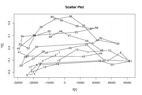
| Dataseries X: | |||||||||||||||||||||||||||||||||||||||||||||||||||||||||||||||||
-3388.23981 -5872.093864 -14052.1039 -19203.67533 -24044.19734 -17742.28074 27744.2042 35762.75709 41087.62968 28606.60883 14902.64899 7759.622726 -3776.912419 -4660.673037 -12883.9742 -20576.76724 -22040.6962 -16004.18577 22072.46441 30238.48835 42118.537 25185.47985 13947.85282 3560.533899 -11669.24371 -13718.99352 -20008.89931 -27883.93174 -25118.66378 -17956.14486 18059.81884 22967.25744 33919.10764 20740.30456 12154.69761 3791.18023 -6213.536375 -15069.58657 -19399.72402 -29503.72248 -28984.08773 -23813.80819 12029.47675 23039.86053 23629.98332 14123.87136 2928.628123 -2532.706238 -9237.265317 -9872.185775 -19113.70932 -23364.3765 -28379.75488 -27061.33248 7441.018864 20404.86134 17037.67756 7876.769459 -2041.972623 -7941.89618 | |||||||||||||||||||||||||||||||||||||||||||||||||||||||||||||||||
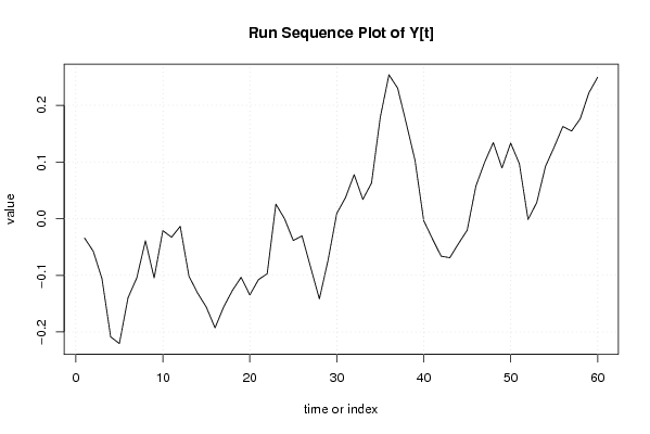
| Dataseries Y: | |||||||||||||||||||||||||||||||||||||||||||||||||||||||||||||||||
-0.034283041 -0.057660003 -0.105996947 -0.208621088 -0.220404198 -0.139474505 -0.104664416 -0.039026785 -0.104663312 -0.021180889 -0.032833113 -0.013625501 -0.101489299 -0.13145901 -0.156198341 -0.19270995 -0.155507653 -0.126748865 -0.103485538 -0.134593206 -0.107595864 -0.097242772 0.025542545 -0.000339608 -0.038608451 -0.030397529 -0.086146589 -0.141688487 -0.073334743 0.009073611 0.03694428 0.077657082 0.0338156 0.062967047 0.178426251 0.253705275 0.230301784 0.167617064 0.102643593 -0.00366903 -0.035648469 -0.066270404 -0.068986516 -0.044020567 -0.020446172 0.057529055 0.099280321 0.134155403 0.089399272 0.133251135 0.096780647 -0.001781812 0.028527049 0.092153397 0.126208459 0.1625611 0.154490341 0.176210215 0.222227014 0.249335133 | |||||||||||||||||||||||||||||||||||||||||||||||||||||||||||||||||
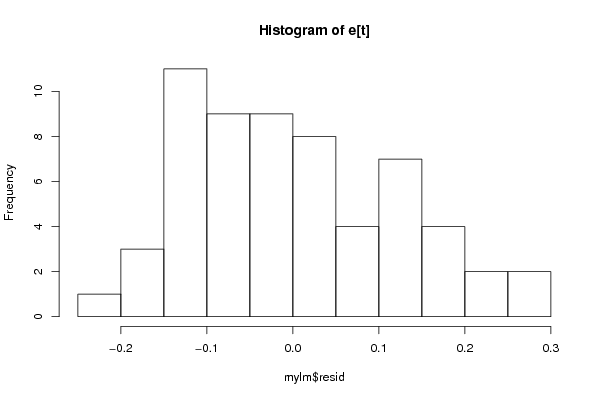
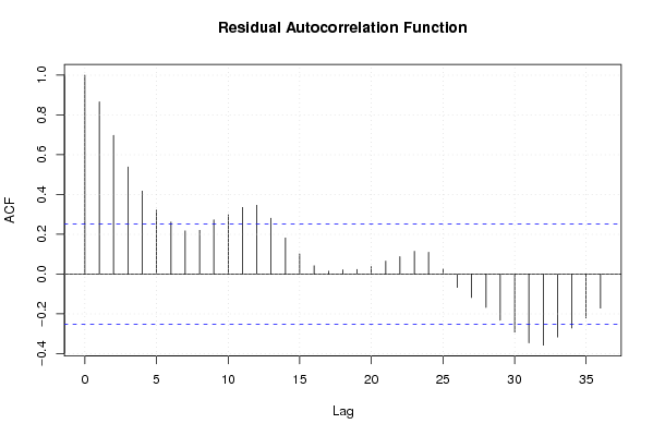
Tables (Output of Computation) | |||||||||||||||||||||||||||||||||||||||||||||||||||||||||||||||||
| |||||||||||||||||||||||||||||||||||||||||||||||||||||||||||||||||
Figures (Output of Computation) | |||||||||||||||||||||||||||||||||||||||||||||||||||||||||||||||||
Input Parameters & R Code | |||||||||||||||||||||||||||||||||||||||||||||||||||||||||||||||||
| Parameters (Session): | |||||||||||||||||||||||||||||||||||||||||||||||||||||||||||||||||
| par1 = 0 ; par2 = 36 ; | |||||||||||||||||||||||||||||||||||||||||||||||||||||||||||||||||
| Parameters (R input): | |||||||||||||||||||||||||||||||||||||||||||||||||||||||||||||||||
| par1 = 0 ; par2 = 36 ; | |||||||||||||||||||||||||||||||||||||||||||||||||||||||||||||||||
| R code (references can be found in the software module): | |||||||||||||||||||||||||||||||||||||||||||||||||||||||||||||||||
par1 <- as.numeric(par1) | |||||||||||||||||||||||||||||||||||||||||||||||||||||||||||||||||