Free Statistics
of Irreproducible Research!
Description of Statistical Computation | |||||||||||||||||||||||||||||||||||||||||||||||||||||||||||||||||
|---|---|---|---|---|---|---|---|---|---|---|---|---|---|---|---|---|---|---|---|---|---|---|---|---|---|---|---|---|---|---|---|---|---|---|---|---|---|---|---|---|---|---|---|---|---|---|---|---|---|---|---|---|---|---|---|---|---|---|---|---|---|---|---|---|---|
| Author's title | |||||||||||||||||||||||||||||||||||||||||||||||||||||||||||||||||
| Author | *Unverified author* | ||||||||||||||||||||||||||||||||||||||||||||||||||||||||||||||||
| R Software Module | rwasp_edabi.wasp | ||||||||||||||||||||||||||||||||||||||||||||||||||||||||||||||||
| Title produced by software | Bivariate Explorative Data Analysis | ||||||||||||||||||||||||||||||||||||||||||||||||||||||||||||||||
| Date of computation | Wed, 28 Oct 2009 06:19:32 -0600 | ||||||||||||||||||||||||||||||||||||||||||||||||||||||||||||||||
| Cite this page as follows | Statistical Computations at FreeStatistics.org, Office for Research Development and Education, URL https://freestatistics.org/blog/index.php?v=date/2009/Oct/28/t1256732455091jlahmono0g2q.htm/, Retrieved Sun, 05 May 2024 22:25:50 +0000 | ||||||||||||||||||||||||||||||||||||||||||||||||||||||||||||||||
| Statistical Computations at FreeStatistics.org, Office for Research Development and Education, URL https://freestatistics.org/blog/index.php?pk=51343, Retrieved Sun, 05 May 2024 22:25:50 +0000 | |||||||||||||||||||||||||||||||||||||||||||||||||||||||||||||||||
| QR Codes: | |||||||||||||||||||||||||||||||||||||||||||||||||||||||||||||||||
|
| |||||||||||||||||||||||||||||||||||||||||||||||||||||||||||||||||
| Original text written by user: | |||||||||||||||||||||||||||||||||||||||||||||||||||||||||||||||||
| IsPrivate? | No (this computation is public) | ||||||||||||||||||||||||||||||||||||||||||||||||||||||||||||||||
| User-defined keywords | |||||||||||||||||||||||||||||||||||||||||||||||||||||||||||||||||
| Estimated Impact | 155 | ||||||||||||||||||||||||||||||||||||||||||||||||||||||||||||||||
Tree of Dependent Computations | |||||||||||||||||||||||||||||||||||||||||||||||||||||||||||||||||
| Family? (F = Feedback message, R = changed R code, M = changed R Module, P = changed Parameters, D = changed Data) | |||||||||||||||||||||||||||||||||||||||||||||||||||||||||||||||||
| F [Trivariate Scatterplots] [trivariate analysis] [2008-11-13 08:14:40] [3b5d63cebdc58ed6c519cdb5b6a36d46] - RMPD [Bivariate Explorative Data Analysis] [college Y=f(Z)] [2009-10-28 12:19:32] [d41d8cd98f00b204e9800998ecf8427e] [Current] - D [Bivariate Explorative Data Analysis] [WS5 berekening Y=...] [2009-10-29 14:37:50] [42ad1186d39724f834063794eac7cea3] - M [Bivariate Explorative Data Analysis] [BDM2] [2009-11-03 11:53:00] [f5d341d4bbba73282fc6e80153a6d315] - M [Bivariate Explorative Data Analysis] [TG2] [2009-11-03 11:59:56] [a21bac9c8d3d56fdec8be4e719e2c7ed] - M [Bivariate Explorative Data Analysis] [P5] [2009-12-15 09:47:24] [f5d341d4bbba73282fc6e80153a6d315] | |||||||||||||||||||||||||||||||||||||||||||||||||||||||||||||||||
| Feedback Forum | |||||||||||||||||||||||||||||||||||||||||||||||||||||||||||||||||
Post a new message | |||||||||||||||||||||||||||||||||||||||||||||||||||||||||||||||||
Dataset | |||||||||||||||||||||||||||||||||||||||||||||||||||||||||||||||||
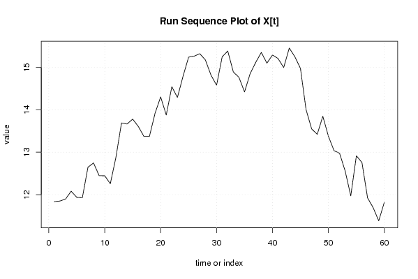
| Dataseries X: | |||||||||||||||||||||||||||||||||||||||||||||||||||||||||||||||||
11.836 11.85 11.897 12.082 11.936 11.928 12.646 12.747 12.447 12.445 12.257 12.878 13.69 13.665 13.78 13.608 13.375 13.376 13.918 14.304 13.877 14.543 14.291 14.788 15.241 15.265 15.322 15.175 14.817 14.579 15.247 15.385 14.891 14.766 14.42 14.85 15.117 15.352 15.099 15.291 15.208 14.995 15.454 15.251 14.975 14.005 13.55 13.422 13.848 13.376 13.038 12.974 12.554 11.971 12.916 12.757 11.924 11.693 11.382 11.821 | |||||||||||||||||||||||||||||||||||||||||||||||||||||||||||||||||
| Dataseries Y: | |||||||||||||||||||||||||||||||||||||||||||||||||||||||||||||||||
3.253 3.233 3.196 3.138 3.091 3.17 3.378 3.468 3.33 3.413 3.356 3.525 3.633 3.597 3.6 3.522 3.503 3.532 3.686 3.748 3.672 3.843 3.905 3.999 4.07 4.084 4.042 3.951 3.933 3.958 4.147 4.221 4.058 4.057 4.089 4.268 4.309 4.303 4.177 4.117 4.065 3.983 4.091 4.067 4.024 3.868 3.8 3.804 3.862 3.792 3.674 3.56 3.489 3.412 3.674 3.672 3.463 3.429 3.4 3.533 | |||||||||||||||||||||||||||||||||||||||||||||||||||||||||||||||||
Tables (Output of Computation) | |||||||||||||||||||||||||||||||||||||||||||||||||||||||||||||||||
| |||||||||||||||||||||||||||||||||||||||||||||||||||||||||||||||||
Figures (Output of Computation) | |||||||||||||||||||||||||||||||||||||||||||||||||||||||||||||||||
Input Parameters & R Code | |||||||||||||||||||||||||||||||||||||||||||||||||||||||||||||||||
| Parameters (Session): | |||||||||||||||||||||||||||||||||||||||||||||||||||||||||||||||||
| par1 = 0 ; par2 = 36 ; | |||||||||||||||||||||||||||||||||||||||||||||||||||||||||||||||||
| Parameters (R input): | |||||||||||||||||||||||||||||||||||||||||||||||||||||||||||||||||
| par1 = 0 ; par2 = 36 ; | |||||||||||||||||||||||||||||||||||||||||||||||||||||||||||||||||
| R code (references can be found in the software module): | |||||||||||||||||||||||||||||||||||||||||||||||||||||||||||||||||
par1 <- as.numeric(par1) | |||||||||||||||||||||||||||||||||||||||||||||||||||||||||||||||||