Free Statistics
of Irreproducible Research!
Description of Statistical Computation | |||||||||||||||||||||
|---|---|---|---|---|---|---|---|---|---|---|---|---|---|---|---|---|---|---|---|---|---|
| Author's title | |||||||||||||||||||||
| Author | *The author of this computation has been verified* | ||||||||||||||||||||
| R Software Module | rwasp_meanplot.wasp | ||||||||||||||||||||
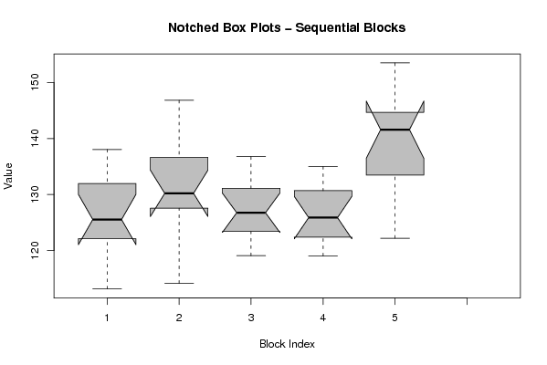
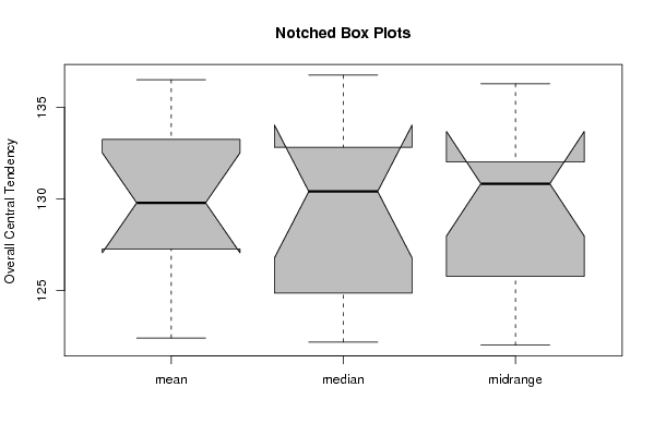
| Title produced by software | Mean Plot | ||||||||||||||||||||
| Date of computation | Fri, 13 Nov 2009 12:40:19 -0700 | ||||||||||||||||||||
| Cite this page as follows | Statistical Computations at FreeStatistics.org, Office for Research Development and Education, URL https://freestatistics.org/blog/index.php?v=date/2009/Nov/13/t12581412867gdgwjlkdcqsapx.htm/, Retrieved Sun, 05 May 2024 10:01:28 +0000 | ||||||||||||||||||||
| Statistical Computations at FreeStatistics.org, Office for Research Development and Education, URL https://freestatistics.org/blog/index.php?pk=57053, Retrieved Sun, 05 May 2024 10:01:28 +0000 | |||||||||||||||||||||
| QR Codes: | |||||||||||||||||||||
|
| |||||||||||||||||||||
| Original text written by user: | |||||||||||||||||||||
| IsPrivate? | No (this computation is public) | ||||||||||||||||||||
| User-defined keywords | bhschhwsstw6l10.4 | ||||||||||||||||||||
| Estimated Impact | 104 | ||||||||||||||||||||
Tree of Dependent Computations | |||||||||||||||||||||
| Family? (F = Feedback message, R = changed R code, M = changed R Module, P = changed Parameters, D = changed Data) | |||||||||||||||||||||
| - [Mean Plot] [3/11/2009] [2009-11-02 22:07:54] [b98453cac15ba1066b407e146608df68] - PD [Mean Plot] [Workshop 6] [2009-11-13 19:40:19] [682632737e024f9e62885141c5f654cd] [Current] | |||||||||||||||||||||
| Feedback Forum | |||||||||||||||||||||
Post a new message | |||||||||||||||||||||
Dataset | |||||||||||||||||||||
| Dataseries X: | |||||||||||||||||||||
126.51 131.02 136.51 138.04 132.92 129.61 122.96 124.04 121.29 124.56 118.53 113.14 114.15 122.17 129.23 131.19 129.12 128.28 126.83 138.13 140.52 146.83 135.14 131.84 125.7 128.98 133.25 136.76 133.24 128.54 121.08 120.23 119.08 125.75 126.89 126.6 121.89 123.44 126.46 129.49 127.78 125.29 119.02 119.96 122.86 131.89 132.73 135.01 136.71 142.73 144.43 144.93 138.75 130.22 122.19 128.4 140.43 153.5 149.33 142.97 | |||||||||||||||||||||
Tables (Output of Computation) | |||||||||||||||||||||
| |||||||||||||||||||||
Figures (Output of Computation) | |||||||||||||||||||||
Input Parameters & R Code | |||||||||||||||||||||
| Parameters (Session): | |||||||||||||||||||||
| par1 = 12 ; | |||||||||||||||||||||
| Parameters (R input): | |||||||||||||||||||||
| par1 = 12 ; | |||||||||||||||||||||
| R code (references can be found in the software module): | |||||||||||||||||||||
par1 <- as.numeric(par1) | |||||||||||||||||||||