Free Statistics
of Irreproducible Research!
Description of Statistical Computation | |||||||||||||||||||||||||||||||||||||||||||||||||||||||||||||||||
|---|---|---|---|---|---|---|---|---|---|---|---|---|---|---|---|---|---|---|---|---|---|---|---|---|---|---|---|---|---|---|---|---|---|---|---|---|---|---|---|---|---|---|---|---|---|---|---|---|---|---|---|---|---|---|---|---|---|---|---|---|---|---|---|---|---|
| Author's title | |||||||||||||||||||||||||||||||||||||||||||||||||||||||||||||||||
| Author | *The author of this computation has been verified* | ||||||||||||||||||||||||||||||||||||||||||||||||||||||||||||||||
| R Software Module | rwasp_edabi.wasp | ||||||||||||||||||||||||||||||||||||||||||||||||||||||||||||||||
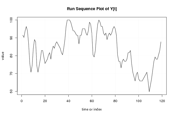
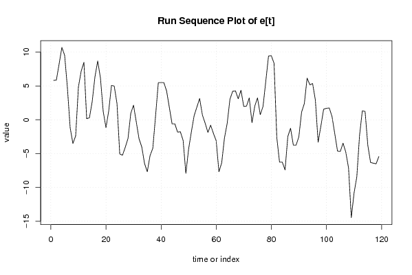
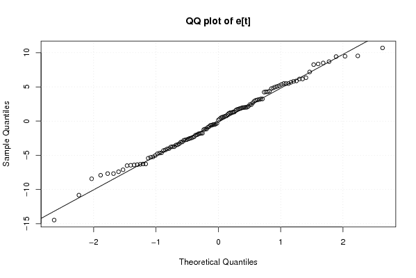
| Title produced by software | Bivariate Explorative Data Analysis | ||||||||||||||||||||||||||||||||||||||||||||||||||||||||||||||||
| Date of computation | Fri, 13 Nov 2009 11:48:03 -0700 | ||||||||||||||||||||||||||||||||||||||||||||||||||||||||||||||||
| Cite this page as follows | Statistical Computations at FreeStatistics.org, Office for Research Development and Education, URL https://freestatistics.org/blog/index.php?v=date/2009/Nov/13/t12581381247jkmk56t5sywkxm.htm/, Retrieved Sun, 05 May 2024 10:37:38 +0000 | ||||||||||||||||||||||||||||||||||||||||||||||||||||||||||||||||
| Statistical Computations at FreeStatistics.org, Office for Research Development and Education, URL https://freestatistics.org/blog/index.php?pk=56995, Retrieved Sun, 05 May 2024 10:37:38 +0000 | |||||||||||||||||||||||||||||||||||||||||||||||||||||||||||||||||
| QR Codes: | |||||||||||||||||||||||||||||||||||||||||||||||||||||||||||||||||
|
| |||||||||||||||||||||||||||||||||||||||||||||||||||||||||||||||||
| Original text written by user: | |||||||||||||||||||||||||||||||||||||||||||||||||||||||||||||||||
| IsPrivate? | No (this computation is public) | ||||||||||||||||||||||||||||||||||||||||||||||||||||||||||||||||
| User-defined keywords | |||||||||||||||||||||||||||||||||||||||||||||||||||||||||||||||||
| Estimated Impact | 215 | ||||||||||||||||||||||||||||||||||||||||||||||||||||||||||||||||
Tree of Dependent Computations | |||||||||||||||||||||||||||||||||||||||||||||||||||||||||||||||||
| Family? (F = Feedback message, R = changed R code, M = changed R Module, P = changed Parameters, D = changed Data) | |||||||||||||||||||||||||||||||||||||||||||||||||||||||||||||||||
| - [Bivariate Explorative Data Analysis] [3/11/2009] [2009-11-02 22:01:32] [b98453cac15ba1066b407e146608df68] - PD [Bivariate Explorative Data Analysis] [ws6 8] [2009-11-13 18:48:03] [d41d8cd98f00b204e9800998ecf8427e] [Current] | |||||||||||||||||||||||||||||||||||||||||||||||||||||||||||||||||
| Feedback Forum | |||||||||||||||||||||||||||||||||||||||||||||||||||||||||||||||||
Post a new message | |||||||||||||||||||||||||||||||||||||||||||||||||||||||||||||||||
Dataset | |||||||||||||||||||||||||||||||||||||||||||||||||||||||||||||||||
| Dataseries X: | |||||||||||||||||||||||||||||||||||||||||||||||||||||||||||||||||
90,70 89,53 90,70 90,70 89,53 87,21 82,56 80,23 82,56 84,88 87,21 84,88 80,23 76,74 77,91 77,91 80,23 82,56 83,72 82,56 81,40 79,07 81,40 84,88 88,37 93,02 94,19 91,86 90,70 90,70 91,86 93,02 93,02 93,02 93,02 94,19 97,67 100,00 98,84 98,84 98,84 98,84 98,84 98,84 98,84 98,84 97,67 98,84 98,84 100,00 97,67 98,84 97,67 96,51 96,51 96,51 100,00 103,49 103,49 100,00 93,02 90,70 90,70 96,51 98,84 100,00 98,84 97,67 96,51 95,35 94,19 94,19 94,19 94,19 94,19 95,35 95,35 94,19 91,86 90,70 88,37 88,37 88,37 88,37 86,05 84,88 84,88 86,05 86,05 86,05 86,05 84,88 82,56 76,74 72,09 72,09 75,58 76,74 75,58 72,09 70,93 72,09 74,42 77,91 79,07 79,07 81,40 79,07 80,23 80,23 81,40 80,23 81,40 83,72 87,21 89,53 91,86 94,19 97,67 | |||||||||||||||||||||||||||||||||||||||||||||||||||||||||||||||||
| Dataseries Y: | |||||||||||||||||||||||||||||||||||||||||||||||||||||||||||||||||
91,46 90,24 93,90 96,34 93,90 86,59 75,61 70,73 74,39 84,15 89,02 87,80 74,39 70,73 74,39 78,05 82,93 82,93 79,27 75,61 76,83 78,05 80,49 81,71 78,05 82,93 85,37 84,15 86,59 87,80 86,59 85,37 84,15 81,71 80,49 84,15 89,02 96,34 100,00 100,00 100,00 98,78 96,34 93,90 93,90 92,68 91,46 91,46 86,59 91,46 91,46 95,12 95,12 95,12 92,68 91,46 93,90 98,78 97,56 92,68 80,49 79,27 82,93 91,46 97,56 100,00 98,78 96,34 96,34 92,68 91,46 92,68 89,02 91,46 92,68 91,46 92,68 95,12 96,34 95,12 91,46 80,49 76,83 76,83 73,17 76,83 78,05 76,83 76,83 78,05 81,71 81,71 82,93 75,61 70,73 68,29 65,85 69,51 70,73 67,07 65,85 65,85 65,85 67,07 68,29 69,51 70,73 65,85 59,76 63,41 67,07 71,95 76,83 79,27 78,05 78,05 80,49 82,93 87,80 | |||||||||||||||||||||||||||||||||||||||||||||||||||||||||||||||||
Tables (Output of Computation) | |||||||||||||||||||||||||||||||||||||||||||||||||||||||||||||||||
| |||||||||||||||||||||||||||||||||||||||||||||||||||||||||||||||||
Figures (Output of Computation) | |||||||||||||||||||||||||||||||||||||||||||||||||||||||||||||||||
Input Parameters & R Code | |||||||||||||||||||||||||||||||||||||||||||||||||||||||||||||||||
| Parameters (Session): | |||||||||||||||||||||||||||||||||||||||||||||||||||||||||||||||||
| par1 = 3 ; par2 = TRUE ; par3 = TRUE ; | |||||||||||||||||||||||||||||||||||||||||||||||||||||||||||||||||
| Parameters (R input): | |||||||||||||||||||||||||||||||||||||||||||||||||||||||||||||||||
| par1 = 0 ; par2 = 36 ; | |||||||||||||||||||||||||||||||||||||||||||||||||||||||||||||||||
| R code (references can be found in the software module): | |||||||||||||||||||||||||||||||||||||||||||||||||||||||||||||||||
par1 <- as.numeric(par1) | |||||||||||||||||||||||||||||||||||||||||||||||||||||||||||||||||