Free Statistics
of Irreproducible Research!
Description of Statistical Computation | |||||||||||||||||||||||||||||||||||||||||||||||||||||||||||||||||
|---|---|---|---|---|---|---|---|---|---|---|---|---|---|---|---|---|---|---|---|---|---|---|---|---|---|---|---|---|---|---|---|---|---|---|---|---|---|---|---|---|---|---|---|---|---|---|---|---|---|---|---|---|---|---|---|---|---|---|---|---|---|---|---|---|---|
| Author's title | |||||||||||||||||||||||||||||||||||||||||||||||||||||||||||||||||
| Author | *The author of this computation has been verified* | ||||||||||||||||||||||||||||||||||||||||||||||||||||||||||||||||
| R Software Module | rwasp_edabi.wasp | ||||||||||||||||||||||||||||||||||||||||||||||||||||||||||||||||
| Title produced by software | Bivariate Explorative Data Analysis | ||||||||||||||||||||||||||||||||||||||||||||||||||||||||||||||||
| Date of computation | Mon, 02 Nov 2009 23:01:32 +0100 | ||||||||||||||||||||||||||||||||||||||||||||||||||||||||||||||||
| Cite this page as follows | Statistical Computations at FreeStatistics.org, Office for Research Development and Education, URL https://freestatistics.org/blog/index.php?v=date/2009/Nov/02/t1257199348qd0w253h76ssio6.htm/, Retrieved Tue, 01 Jul 2025 02:48:22 +0000 | ||||||||||||||||||||||||||||||||||||||||||||||||||||||||||||||||
| Statistical Computations at FreeStatistics.org, Office for Research Development and Education, URL https://freestatistics.org/blog/index.php?pk=53030, Retrieved Tue, 01 Jul 2025 02:48:22 +0000 | |||||||||||||||||||||||||||||||||||||||||||||||||||||||||||||||||
| QR Codes: | |||||||||||||||||||||||||||||||||||||||||||||||||||||||||||||||||
|
| |||||||||||||||||||||||||||||||||||||||||||||||||||||||||||||||||
| Original text written by user: | |||||||||||||||||||||||||||||||||||||||||||||||||||||||||||||||||
| IsPrivate? | No (this computation is public) | ||||||||||||||||||||||||||||||||||||||||||||||||||||||||||||||||
| User-defined keywords | |||||||||||||||||||||||||||||||||||||||||||||||||||||||||||||||||
| Estimated Impact | 683 | ||||||||||||||||||||||||||||||||||||||||||||||||||||||||||||||||
Tree of Dependent Computations | |||||||||||||||||||||||||||||||||||||||||||||||||||||||||||||||||
| Family? (F = Feedback message, R = changed R code, M = changed R Module, P = changed Parameters, D = changed Data) | |||||||||||||||||||||||||||||||||||||||||||||||||||||||||||||||||
| - [Bivariate Explorative Data Analysis] [3/11/2009] [2009-11-02 22:01:32] [d76b387543b13b5e3afd8ff9e5fdc89f] [Current] - PD [Bivariate Explorative Data Analysis] [] [2009-11-04 15:37:15] [8d2349dc1d6314bc274adc9ad027c980] - PD [Bivariate Explorative Data Analysis] [] [2009-11-04 15:40:15] [4d62210f0915d3a20cbf115865da7cd4] - R PD [Bivariate Explorative Data Analysis] [bivariate EDA] [2009-11-04 15:39:01] [757146c69eaf0537be37c7b0c18216d8] - PD [Bivariate Explorative Data Analysis] [e] [2009-11-04 19:19:29] [315ba876df544ad397193b5931d5f354] - PD [Bivariate Explorative Data Analysis] [e] [2009-11-04 19:19:29] [315ba876df544ad397193b5931d5f354] - PD [Bivariate Explorative Data Analysis] [e] [2009-11-04 19:19:29] [315ba876df544ad397193b5931d5f354] - PD [Bivariate Explorative Data Analysis] [e] [2009-11-04 19:19:29] [315ba876df544ad397193b5931d5f354] - PD [Bivariate Explorative Data Analysis] [e] [2009-11-04 19:19:29] [315ba876df544ad397193b5931d5f354] - PD [Bivariate Explorative Data Analysis] [e] [2009-11-04 19:19:29] [315ba876df544ad397193b5931d5f354] - P [Bivariate Explorative Data Analysis] [Paper] [2009-12-09 19:12:24] [3e19a07d230ba260a720e0e03e0f40f2] - PD [Bivariate Explorative Data Analysis] [e] [2009-11-04 19:19:29] [315ba876df544ad397193b5931d5f354] - D [Bivariate Explorative Data Analysis] [ws 6 cb] [2009-11-04 22:31:43] [6e4e01d7eb22a9f33d58ebb35753a195] - PD [Bivariate Explorative Data Analysis] [bivariate EDA] [2009-11-05 10:39:22] [cd6314e7e707a6546bd4604c9d1f2b69] - PD [Bivariate Explorative Data Analysis] [SHW WS6 - Regress...] [2009-11-05 10:40:51] [253127ae8da904b75450fbd69fe4eb21] - D [Bivariate Explorative Data Analysis] [SHW WS6 - Review ...] [2009-11-15 11:41:40] [253127ae8da904b75450fbd69fe4eb21] - PD [Bivariate Explorative Data Analysis] [SHW WS6 - Regress...] [2009-12-13 09:48:02] [253127ae8da904b75450fbd69fe4eb21] - RMPD [Mean Plot] [SHW WS6 - Mean Plot] [2009-11-05 10:45:27] [253127ae8da904b75450fbd69fe4eb21] - [Mean Plot] [SHW WS6 - Mean Plot] [2009-12-13 13:51:12] [253127ae8da904b75450fbd69fe4eb21] - D [Bivariate Explorative Data Analysis] [WS 6 Bivariate ED...] [2009-11-05 10:47:30] [b103a1dc147def8132c7f643ad8c8f84] - RMPD [Standard Deviation Plot] [SHW WS6 - Standar...] [2009-11-05 10:48:09] [253127ae8da904b75450fbd69fe4eb21] - RMPD [Standard Deviation Plot] [SHW WS6 - Tukey l...] [2009-11-05 10:48:09] [253127ae8da904b75450fbd69fe4eb21] - PD [Bivariate Explorative Data Analysis] [Bivariate EDA Wer...] [2009-11-05 12:06:49] [4395c69e961f9a13a0559fd2f0a72538] - PD [Bivariate Explorative Data Analysis] [Workshop 6] [2009-11-05 12:32:58] [03557919bc1ce1475f4920f6a43c36b0] - PD [Bivariate Explorative Data Analysis] [Assumpties BDM] [2009-11-05 13:08:56] [f5d341d4bbba73282fc6e80153a6d315] - PD [Bivariate Explorative Data Analysis] [Shwws6v1] [2009-11-05 14:30:47] [5f89c040fdf1f8599c99d7f78a662321] - PD [Bivariate Explorative Data Analysis] [shwws6vr1] [2009-11-05 14:30:49] [2b2cfeea2f5ac2a1bcb842baaf1415ef] - PD [Bivariate Explorative Data Analysis] [run sequence plot] [2009-11-05 15:47:03] [eaf42bcf5162b5692bb3c7f9d4636222] - D [Bivariate Explorative Data Analysis] [shw6: Bivariate EDA] [2009-11-05 19:05:09] [3c8b83428ce260cd44df892bb7619588] - PD [Bivariate Explorative Data Analysis] [] [2009-11-06 10:48:02] [74be16979710d4c4e7c6647856088456] - PD [Bivariate Explorative Data Analysis] [Workshop 6] [2009-11-06 13:55:46] [786e067c4f7cec17385c4742b96b6dfa] - PD [Bivariate Explorative Data Analysis] [Workshop 6] [2009-11-06 13:59:02] [786e067c4f7cec17385c4742b96b6dfa] - PD [Bivariate Explorative Data Analysis] [ws 6] [2009-11-07 13:34:21] [b5908418e3090fddbd22f5f0f774653d] - PD [Bivariate Explorative Data Analysis] [Bivariate analyse] [2009-11-07 14:19:18] [d46757a0a8c9b00540ab7e7e0c34bfc4] - PD [Bivariate Explorative Data Analysis] [] [2009-11-07 14:56:46] [2f674a53c3d7aaa1bcf80e66074d3c9b] - D [Bivariate Explorative Data Analysis] [WS 6: Bivariate EDA] [2009-11-07 16:03:55] [8cf9233b7464ea02e32be3b30fdac052] - PD [Bivariate Explorative Data Analysis] [WS 6: Bivariate EDA] [2009-11-12 17:13:47] [b97b96148b0223bc16666763988dc147] - PD [Bivariate Explorative Data Analysis] [SHWWS6link9] [2009-11-08 10:12:52] [a66d3a79ef9e5308cd94a469bc5ca464] - RM D [Kendall tau Correlation Matrix] [] [2009-11-08 14:22:16] [7369a9baefff1ba9d2171738b4c9faa6] F PD [Bivariate Explorative Data Analysis] [] [2009-11-08 16:17:02] [cf890101a20378422561610e0d41fd9c] - D [Bivariate Explorative Data Analysis] [Regressierechte] [2009-11-08 16:25:45] [e2a6b1b31bd881219e1879835b4c60d0] - PD [Bivariate Explorative Data Analysis] [Regressierechte] [2009-12-13 19:32:48] [e2a6b1b31bd881219e1879835b4c60d0] - D [Bivariate Explorative Data Analysis] [Regressierechte] [2009-12-13 19:42:44] [e2a6b1b31bd881219e1879835b4c60d0] - PD [Bivariate Explorative Data Analysis] [WS 6 EDA Y[t] = c...] [2009-11-09 09:33:21] [83058a88a37d754675a5cd22dab372fc] - PD [Bivariate Explorative Data Analysis] [workshop 6] [2009-11-09 09:50:28] [3e19a07d230ba260a720e0e03e0f40f2] - PD [Bivariate Explorative Data Analysis] [Bivariate EDA icv...] [2009-11-09 10:41:13] [134dc66689e3d457a82860db6471d419] - PD [Bivariate Explorative Data Analysis] [Bivariate EDA icp...] [2009-11-09 10:56:58] [134dc66689e3d457a82860db6471d419] - PD [Bivariate Explorative Data Analysis] [WS 6: Bivariate EDA] [2009-11-09 12:55:21] [74be16979710d4c4e7c6647856088456] - PD [Bivariate Explorative Data Analysis] [] [2009-11-09 18:21:28] [ee35698a38947a6c6c039b1e3deafc05] [Truncated] | |||||||||||||||||||||||||||||||||||||||||||||||||||||||||||||||||
| Feedback Forum | |||||||||||||||||||||||||||||||||||||||||||||||||||||||||||||||||
Post a new message | |||||||||||||||||||||||||||||||||||||||||||||||||||||||||||||||||
Dataset | |||||||||||||||||||||||||||||||||||||||||||||||||||||||||||||||||
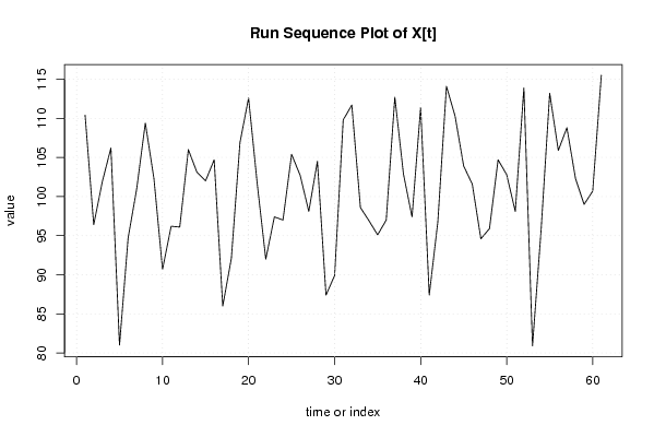
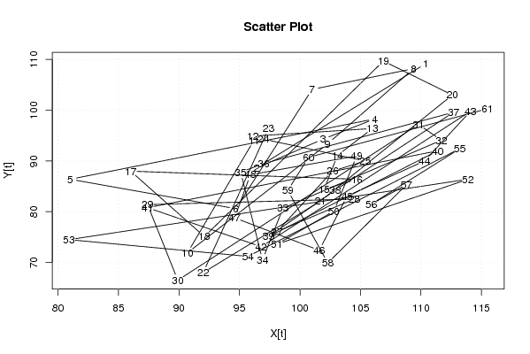
| Dataseries X: | |||||||||||||||||||||||||||||||||||||||||||||||||||||||||||||||||
110.40 96.40 101.90 106.20 81.00 94.70 101.00 109.40 102.30 90.70 96.20 96.10 106.00 103.10 102.00 104.70 86.00 92.10 106.90 112.60 101.70 92.00 97.40 97.00 105.40 102.70 98.10 104.50 87.40 89.90 109.80 111.70 98.60 96.90 95.10 97.00 112.70 102.90 97.40 111.40 87.40 96.80 114.10 110.30 103.90 101.60 94.60 95.90 104.70 102.80 98.10 113.90 80.90 95.70 113.20 105.90 108.80 102.30 99.00 100.70 115.50 | |||||||||||||||||||||||||||||||||||||||||||||||||||||||||||||||||
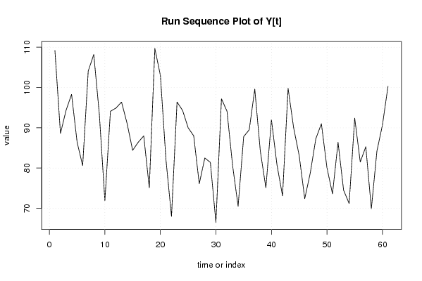
| Dataseries Y: | |||||||||||||||||||||||||||||||||||||||||||||||||||||||||||||||||
109.20 88.60 94.30 98.30 86.40 80.60 104.10 108.20 93.40 71.90 94.10 94.90 96.40 91.10 84.40 86.40 88.00 75.10 109.70 103.00 82.10 68.00 96.40 94.30 90.00 88.00 76.10 82.50 81.40 66.50 97.20 94.10 80.70 70.50 87.80 89.50 99.60 84.20 75.10 92.00 80.80 73.10 99.80 90.00 83.10 72.40 78.80 87.30 91.00 80.10 73.60 86.40 74.50 71.20 92.40 81.50 85.30 69.90 84.20 90.70 100.30 | |||||||||||||||||||||||||||||||||||||||||||||||||||||||||||||||||
Tables (Output of Computation) | |||||||||||||||||||||||||||||||||||||||||||||||||||||||||||||||||
| |||||||||||||||||||||||||||||||||||||||||||||||||||||||||||||||||
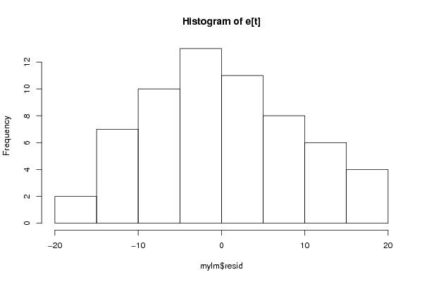
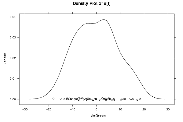
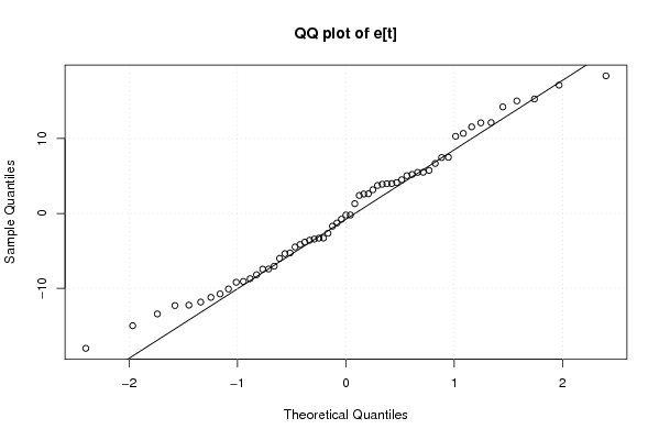
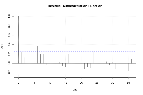
Figures (Output of Computation) | |||||||||||||||||||||||||||||||||||||||||||||||||||||||||||||||||
Input Parameters & R Code | |||||||||||||||||||||||||||||||||||||||||||||||||||||||||||||||||
| Parameters (Session): | |||||||||||||||||||||||||||||||||||||||||||||||||||||||||||||||||
| Parameters (R input): | |||||||||||||||||||||||||||||||||||||||||||||||||||||||||||||||||
| par1 = 0 ; par2 = 36 ; | |||||||||||||||||||||||||||||||||||||||||||||||||||||||||||||||||
| R code (references can be found in the software module): | |||||||||||||||||||||||||||||||||||||||||||||||||||||||||||||||||
par1 <- as.numeric(par1) | |||||||||||||||||||||||||||||||||||||||||||||||||||||||||||||||||