Repository of Reproducible Computations

Free Statistics

of Irreproducible Research!

Author's title

Author

*The author of this computation has been verified*

R Software Module

rwasp_notchedbox1.wasp

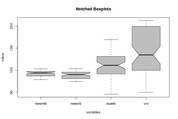
Title produced by software

Notched Boxplots

Date of computation

Fri, 13 Nov 2009 08:17:37 -0700

Cite this page as follows

Statistical Computations at FreeStatistics.org, Office for Research Development and Education, URL https://freestatistics.org/blog/index.php?v=date/2009/Nov/13/t1258125566qx5pimr93b1i0x7.htm/, Retrieved Sun, 05 May 2024 18:10:31 +0000

Statistical Computations at FreeStatistics.org, Office for Research Development and Education, URL https://freestatistics.org/blog/index.php?pk=56802, Retrieved Sun, 05 May 2024 18:10:31 +0000

QR Codes:

Paste this QR Code to cite your computation.

Original text written by user:

IsPrivate?

No (this computation is public)

User-defined keywords

WS 6

Estimated Impact

190

Family? (F = Feedback message, R = changed R code, M = changed R Module, P = changed Parameters, D = changed Data)

-     [Notched Boxplots] [3/11/2009] [2009-11-02 21:10:41] [b98453cac15ba1066b407e146608df68]
-    D  [Notched Boxplots] [WS 6] [2009-11-13 14:58:42] [9717cb857c153ca3061376906953b329]
-    D      [Notched Boxplots] [WS 6] [2009-11-13 15:17:37] [52b85b290d6f50b0921ad6729b8a5af2] [Current]

Feedback Forum

Post a new message

Dataseries X:

Download CSV

Histogram

Boxplots

100,00	100,00	100,00	100,00
98,76	100,70	111,86	100,00
96,54	97,38	94,12	100,00
96,97	97,40	67,79	100,00
96,69	96,24	146,04	100,00
96,69	95,79	125,66	100,00
95,96	94,90	142,87	100,00
94,26	92,93	130,03	100,00
93,21	92,12	110,01	100,00
92,46	93,26	132,79	100,00
100,23	102,29	88,24	100,00
101,60	103,58	91,97	100,00
101,99	103,04	96,65	100,00
100,55	99,36	97,15	100,00
98,21	96,29	90,73	100,00
98,62	96,46	52,53	110,50
97,76	96,08	156,91	112,50
97,84	94,99	144,88	112,50
96,59	92,93	169,43	122,50
96,03	91,71	133,38	125,00
95,73	91,54	131,28	125,00
94,66	92,52	116,33	132,00
101,12	101,15	89,15	137,50
101,44	102,78	85,08	146,50
101,99	100,49	89,39	150,00
97,18	94,82	103,09	158,50
94,15	90,77	85,35	162,50
92,76	89,39	45,99	169,50
93,87	89,43	152,82	175,00
92,18	87,32	130,37	175,00
89,04	84,81	150,50	182,50
88,40	83,61	126,97	187,50
85,85	81,28	123,24	187,50
82,13	80,76	126,57	195,00
90,21	91,04	100,26	200,00
91,06	93,13	91,76	200,00
88,86	88,03	100,28	200,00
87,45	84,79	121,65	200,00
84,93	81,72	97,29	200,00
86,22	81,95	62,55	200,00
86,72	82,32	154,99	200,00
85,50	80,53	147,85	200,00
82,72	78,38	147,40	200,00
82,72	77,65	156,80	200,00
78,70	74,78	126,81	200,00
79,15	76,91	131,76	200,00
86,51	86,02	99,21	209,00
86,65	87,50	87,35	212,50
86,17	83,12	100,76	212,50
85,52	80,08	110,57	198,50
85,93	78,40	76,46	171,00
89,24	79,87	56,51	137,50
92,23	80,95	124,95	115,50
93,63	81,07	118,29	100,00
95,27	80,76	136,43	83,00
95,59	80,54	128,62	65,50
93,31	78,58	100,74	54,50
94,90	81,05	111,75	50,00
102,13	90,14	93,43	50,00
103,24	92,24	83,33	50,00

Summary of computational transaction
Raw Input	view raw input (R code)
Raw Output	view raw output of R engine
Computing time	1 seconds
R Server	'Gwilym Jenkins' @ 72.249.127.135

\begin{tabular}{lllllllll}
\hline
Summary of computational transaction \tabularnewline
Raw Input & view raw input (R code)  \tabularnewline
Raw Output & view raw output of R engine  \tabularnewline
Computing time & 1 seconds \tabularnewline
R Server & 'Gwilym Jenkins' @ 72.249.127.135 \tabularnewline
\hline
\end{tabular}
%Source: https://freestatistics.org/blog/index.php?pk=56802&T=0

[TABLE]
[ROW][C]Summary of computational transaction[/C][/ROW]
[ROW][C]Raw Input[/C][C]view raw input (R code) [/C][/ROW]
[ROW][C]Raw Output[/C][C]view raw output of R engine [/C][/ROW]
[ROW][C]Computing time[/C][C]1 seconds[/C][/ROW]
[ROW][C]R Server[/C][C]'Gwilym Jenkins' @ 72.249.127.135[/C][/ROW]
[/TABLE]
Source: https://freestatistics.org/blog/index.php?pk=56802&T=0

Globally Unique Identifier (entire table): ba.freestatistics.org/blog/index.php?pk=56802&T=0

As an alternative you can also use a QR Code:

The GUIDs for individual cells are displayed in the table below:

Summary of computational transaction
Raw Input	view raw input (R code)
Raw Output	view raw output of R engine
Computing time	1 seconds
R Server	'Gwilym Jenkins' @ 72.249.127.135

Boxplot statistics
Variable	lower whisker	lower hinge	median	upper hinge	upper whisker
nwwmb	78.7	87.085	94.01	97.47	103.24
nwwvb	74.78	81.175	90.455	95.935	103.58
inpwb	45.99	91.865	111.16	131.52	169.43
vrv	50	100	134.75	199.25	212.5

\begin{tabular}{lllllllll}
\hline
Boxplot statistics \tabularnewline
Variable & lower whisker & lower hinge & median & upper hinge & upper whisker \tabularnewline
nwwmb & 78.7 & 87.085 & 94.01 & 97.47 & 103.24 \tabularnewline
nwwvb & 74.78 & 81.175 & 90.455 & 95.935 & 103.58 \tabularnewline
inpwb & 45.99 & 91.865 & 111.16 & 131.52 & 169.43 \tabularnewline
vrv & 50 & 100 & 134.75 & 199.25 & 212.5 \tabularnewline
\hline
\end{tabular}
%Source: https://freestatistics.org/blog/index.php?pk=56802&T=1

[TABLE]
[ROW][C]Boxplot statistics[/C][/ROW]
[ROW][C]Variable[/C][C]lower whisker[/C][C]lower hinge[/C][C]median[/C][C]upper hinge[/C][C]upper whisker[/C][/ROW]
[ROW][C]nwwmb[/C][C]78.7[/C][C]87.085[/C][C]94.01[/C][C]97.47[/C][C]103.24[/C][/ROW]
[ROW][C]nwwvb[/C][C]74.78[/C][C]81.175[/C][C]90.455[/C][C]95.935[/C][C]103.58[/C][/ROW]
[ROW][C]inpwb[/C][C]45.99[/C][C]91.865[/C][C]111.16[/C][C]131.52[/C][C]169.43[/C][/ROW]
[ROW][C]vrv[/C][C]50[/C][C]100[/C][C]134.75[/C][C]199.25[/C][C]212.5[/C][/ROW]
[/TABLE]
Source: https://freestatistics.org/blog/index.php?pk=56802&T=1

Globally Unique Identifier (entire table): ba.freestatistics.org/blog/index.php?pk=56802&T=1

As an alternative you can also use a QR Code:

The GUIDs for individual cells are displayed in the table below:

Boxplot statistics
Variable	lower whisker	lower hinge	median	upper hinge	upper whisker
nwwmb	78.7	87.085	94.01	97.47	103.24
nwwvb	74.78	81.175	90.455	95.935	103.58
inpwb	45.99	91.865	111.16	131.52	169.43
vrv	50	100	134.75	199.25	212.5

Boxplot Notches
Variable	lower bound	median	upper bound
nwwmb	91.8916975786808	94.01	96.1283024213192
nwwvb	87.4442976659922	90.455	93.4657023340078
inpwb	103.071287191390	111.16	119.248712808610
vrv	114.505270552149	134.75	154.994729447851

\begin{tabular}{lllllllll}
\hline
Boxplot Notches \tabularnewline
Variable & lower bound & median & upper bound \tabularnewline
nwwmb & 91.8916975786808 & 94.01 & 96.1283024213192 \tabularnewline
nwwvb & 87.4442976659922 & 90.455 & 93.4657023340078 \tabularnewline
inpwb & 103.071287191390 & 111.16 & 119.248712808610 \tabularnewline
vrv & 114.505270552149 & 134.75 & 154.994729447851 \tabularnewline
\hline
\end{tabular}
%Source: https://freestatistics.org/blog/index.php?pk=56802&T=2

[TABLE]
[ROW][C]Boxplot Notches[/C][/ROW]
[ROW][C]Variable[/C][C]lower bound[/C][C]median[/C][C]upper bound[/C][/ROW]
[ROW][C]nwwmb[/C][C]91.8916975786808[/C][C]94.01[/C][C]96.1283024213192[/C][/ROW]
[ROW][C]nwwvb[/C][C]87.4442976659922[/C][C]90.455[/C][C]93.4657023340078[/C][/ROW]
[ROW][C]inpwb[/C][C]103.071287191390[/C][C]111.16[/C][C]119.248712808610[/C][/ROW]
[ROW][C]vrv[/C][C]114.505270552149[/C][C]134.75[/C][C]154.994729447851[/C][/ROW]
[/TABLE]
Source: https://freestatistics.org/blog/index.php?pk=56802&T=2

Globally Unique Identifier (entire table): ba.freestatistics.org/blog/index.php?pk=56802&T=2

As an alternative you can also use a QR Code:

The GUIDs for individual cells are displayed in the table below:

Boxplot Notches
Variable	lower bound	median	upper bound
nwwmb	91.8916975786808	94.01	96.1283024213192
nwwvb	87.4442976659922	90.455	93.4657023340078
inpwb	103.071287191390	111.16	119.248712808610
vrv	114.505270552149	134.75	154.994729447851

Figure 1

PNG link

Postscript link

PDF link

Parameters (Session):

par1 = grey ;

Parameters (R input):

par1 = grey ;

R code (references can be found in the software module):

z <- as.data.frame(t(y))
bitmap(file='test1.png')
(r<-boxplot(z ,xlab=xlab,ylab=ylab,main=main,notch=TRUE,col=par1))
dev.off()
load(file='createtable')
a<-table.start()
a<-table.row.start(a)
a<-table.element(a,hyperlink('overview.htm','Boxplot statistics','Boxplot overview'),6,TRUE)
a<-table.row.end(a)
a<-table.row.start(a)
a<-table.element(a,'Variable',1,TRUE)
a<-table.element(a,hyperlink('lower_whisker.htm','lower whisker','definition of lower whisker'),1,TRUE)
a<-table.element(a,hyperlink('lower_hinge.htm','lower hinge','definition of lower hinge'),1,TRUE)
a<-table.element(a,hyperlink('central_tendency.htm','median','definitions about measures of central tendency'),1,TRUE)
a<-table.element(a,hyperlink('upper_hinge.htm','upper hinge','definition of upper hinge'),1,TRUE)
a<-table.element(a,hyperlink('upper_whisker.htm','upper whisker','definition of upper whisker'),1,TRUE)
a<-table.row.end(a)
for (i in 1:length(y[,1]))
{
a<-table.row.start(a)
a<-table.element(a,dimnames(t(x))[[2]][i],1,TRUE)
for (j in 1:5)
{
a<-table.element(a,r$stats[j,i])
}
a<-table.row.end(a)
}
a<-table.end(a)
table.save(a,file='mytable.tab')
a<-table.start()
a<-table.row.start(a)
a<-table.element(a,'Boxplot Notches',4,TRUE)
a<-table.row.end(a)
a<-table.row.start(a)
a<-table.element(a,'Variable',1,TRUE)
a<-table.element(a,'lower bound',1,TRUE)
a<-table.element(a,'median',1,TRUE)
a<-table.element(a,'upper bound',1,TRUE)
a<-table.row.end(a)
for (i in 1:length(y[,1]))
{
a<-table.row.start(a)
a<-table.element(a,dimnames(t(x))[[2]][i],1,TRUE)
a<-table.element(a,r$conf[1,i])
a<-table.element(a,r$stats[3,i])
a<-table.element(a,r$conf[2,i])
a<-table.row.end(a)
}
a<-table.end(a)
table.save(a,file='mytable1.tab')

Free Statistics

Description of Statistical Computation

Tree of Dependent Computations

Dataset

Tables (Output of Computation)

Figures (Output of Computation)

Input Parameters & R Code