Free Statistics
of Irreproducible Research!
Description of Statistical Computation | |||||||||||||||||||||||||||||||||||||||||||||||||||||||||||||||||
|---|---|---|---|---|---|---|---|---|---|---|---|---|---|---|---|---|---|---|---|---|---|---|---|---|---|---|---|---|---|---|---|---|---|---|---|---|---|---|---|---|---|---|---|---|---|---|---|---|---|---|---|---|---|---|---|---|---|---|---|---|---|---|---|---|---|
| Author's title | |||||||||||||||||||||||||||||||||||||||||||||||||||||||||||||||||
| Author | *The author of this computation has been verified* | ||||||||||||||||||||||||||||||||||||||||||||||||||||||||||||||||
| R Software Module | rwasp_edabi.wasp | ||||||||||||||||||||||||||||||||||||||||||||||||||||||||||||||||
| Title produced by software | Bivariate Explorative Data Analysis | ||||||||||||||||||||||||||||||||||||||||||||||||||||||||||||||||
| Date of computation | Thu, 12 Nov 2009 06:53:12 -0700 | ||||||||||||||||||||||||||||||||||||||||||||||||||||||||||||||||
| Cite this page as follows | Statistical Computations at FreeStatistics.org, Office for Research Development and Education, URL https://freestatistics.org/blog/index.php?v=date/2009/Nov/12/t1258034052ho7s8phypxrlwyv.htm/, Retrieved Fri, 03 May 2024 19:39:47 +0000 | ||||||||||||||||||||||||||||||||||||||||||||||||||||||||||||||||
| Statistical Computations at FreeStatistics.org, Office for Research Development and Education, URL https://freestatistics.org/blog/index.php?pk=55982, Retrieved Fri, 03 May 2024 19:39:47 +0000 | |||||||||||||||||||||||||||||||||||||||||||||||||||||||||||||||||
| QR Codes: | |||||||||||||||||||||||||||||||||||||||||||||||||||||||||||||||||
|
| |||||||||||||||||||||||||||||||||||||||||||||||||||||||||||||||||
| Original text written by user: | |||||||||||||||||||||||||||||||||||||||||||||||||||||||||||||||||
| IsPrivate? | No (this computation is public) | ||||||||||||||||||||||||||||||||||||||||||||||||||||||||||||||||
| User-defined keywords | |||||||||||||||||||||||||||||||||||||||||||||||||||||||||||||||||
| Estimated Impact | 131 | ||||||||||||||||||||||||||||||||||||||||||||||||||||||||||||||||
Tree of Dependent Computations | |||||||||||||||||||||||||||||||||||||||||||||||||||||||||||||||||
| Family? (F = Feedback message, R = changed R code, M = changed R Module, P = changed Parameters, D = changed Data) | |||||||||||||||||||||||||||||||||||||||||||||||||||||||||||||||||
| - [Bivariate Explorative Data Analysis] [3/11/2009] [2009-11-02 22:01:32] [b98453cac15ba1066b407e146608df68] - PD [Bivariate Explorative Data Analysis] [] [2009-11-12 13:53:12] [4672b66a35a4d755714bdcf00037725e] [Current] - D [Bivariate Explorative Data Analysis] [] [2009-12-15 15:53:24] [73863f7f907331e734eff34b7de6fc83] | |||||||||||||||||||||||||||||||||||||||||||||||||||||||||||||||||
| Feedback Forum | |||||||||||||||||||||||||||||||||||||||||||||||||||||||||||||||||
Post a new message | |||||||||||||||||||||||||||||||||||||||||||||||||||||||||||||||||
Dataset | |||||||||||||||||||||||||||||||||||||||||||||||||||||||||||||||||
| Dataseries X: | |||||||||||||||||||||||||||||||||||||||||||||||||||||||||||||||||
1,43 1,43 1,43 1,43 1,43 1,43 1,43 1,43 1,43 1,43 1,43 1,43 1,43 1,43 1,43 1,43 1,43 1,43 1,44 1,48 1,48 1,48 1,48 1,48 1,48 1,48 1,48 1,48 1,48 1,48 1,48 1,48 1,48 1,48 1,48 1,48 1,48 1,48 1,48 1,48 1,48 1,48 1,48 1,48 1,48 1,48 1,48 1,48 1,48 1,57 1,58 1,58 1,58 1,58 1,59 1,6 1,6 1,61 1,61 1,61 1,62 1,63 1,63 1,64 1,64 1,64 1,64 1,64 1,65 1,65 1,65 1,65 | |||||||||||||||||||||||||||||||||||||||||||||||||||||||||||||||||
| Dataseries Y: | |||||||||||||||||||||||||||||||||||||||||||||||||||||||||||||||||
0,3 2,1 2,5 2,3 2,4 3 1,7 3,5 4 3,7 3,7 3 2,7 2,5 2,2 2,9 3,1 3 2,8 2,5 1,9 1,9 1,8 2 2,6 2,5 2,5 1,6 1,4 0,8 1,1 1,3 1,2 1,3 1,1 1,3 1,2 1,6 1,7 1,5 0,9 1,5 1,4 1,6 1,7 1,4 1,8 1,7 1,4 1,2 1 1,7 2,4 2 2,1 2 1,8 2,7 2,3 1,9 2 2,3 2,8 2,4 2,3 2,7 2,7 2,9 3 2,2 2,3 2,8 | |||||||||||||||||||||||||||||||||||||||||||||||||||||||||||||||||
Tables (Output of Computation) | |||||||||||||||||||||||||||||||||||||||||||||||||||||||||||||||||
| |||||||||||||||||||||||||||||||||||||||||||||||||||||||||||||||||
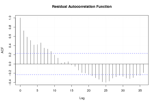
Figures (Output of Computation) | |||||||||||||||||||||||||||||||||||||||||||||||||||||||||||||||||
Input Parameters & R Code | |||||||||||||||||||||||||||||||||||||||||||||||||||||||||||||||||
| Parameters (Session): | |||||||||||||||||||||||||||||||||||||||||||||||||||||||||||||||||
| par1 = 0 ; par2 = 36 ; | |||||||||||||||||||||||||||||||||||||||||||||||||||||||||||||||||
| Parameters (R input): | |||||||||||||||||||||||||||||||||||||||||||||||||||||||||||||||||
| par1 = 0 ; par2 = 36 ; | |||||||||||||||||||||||||||||||||||||||||||||||||||||||||||||||||
| R code (references can be found in the software module): | |||||||||||||||||||||||||||||||||||||||||||||||||||||||||||||||||
par1 <- as.numeric(par1) | |||||||||||||||||||||||||||||||||||||||||||||||||||||||||||||||||