Free Statistics
of Irreproducible Research!
Description of Statistical Computation | |||||||||||||||||||||
|---|---|---|---|---|---|---|---|---|---|---|---|---|---|---|---|---|---|---|---|---|---|
| Author's title | |||||||||||||||||||||
| Author | *The author of this computation has been verified* | ||||||||||||||||||||
| R Software Module | rwasp_meanplot.wasp | ||||||||||||||||||||
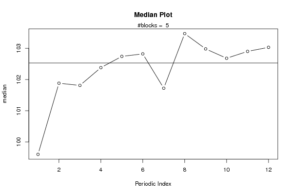
| Title produced by software | Mean Plot | ||||||||||||||||||||
| Date of computation | Thu, 12 Nov 2009 03:35:34 -0700 | ||||||||||||||||||||
| Cite this page as follows | Statistical Computations at FreeStatistics.org, Office for Research Development and Education, URL https://freestatistics.org/blog/index.php?v=date/2009/Nov/12/t12580223509m17da66dhxul3w.htm/, Retrieved Fri, 03 May 2024 22:20:36 +0000 | ||||||||||||||||||||
| Statistical Computations at FreeStatistics.org, Office for Research Development and Education, URL https://freestatistics.org/blog/index.php?pk=55925, Retrieved Fri, 03 May 2024 22:20:36 +0000 | |||||||||||||||||||||
| QR Codes: | |||||||||||||||||||||
|
| |||||||||||||||||||||
| Original text written by user: | |||||||||||||||||||||
| IsPrivate? | No (this computation is public) | ||||||||||||||||||||
| User-defined keywords | |||||||||||||||||||||
| Estimated Impact | 204 | ||||||||||||||||||||
Tree of Dependent Computations | |||||||||||||||||||||
| Family? (F = Feedback message, R = changed R code, M = changed R Module, P = changed Parameters, D = changed Data) | |||||||||||||||||||||
| - [Mean Plot] [3/11/2009] [2009-11-02 22:07:54] [b98453cac15ba1066b407e146608df68] - PD [Mean Plot] [] [2009-11-12 10:35:34] [873be88d67c17ca20f1ec7e5d8eb10d1] [Current] - D [Mean Plot] [] [2009-11-12 10:42:49] [94b62ad0aa784646217b93aa983cee13] | |||||||||||||||||||||
| Feedback Forum | |||||||||||||||||||||
Post a new message | |||||||||||||||||||||
Dataset | |||||||||||||||||||||
| Dataseries X: | |||||||||||||||||||||
95.05 96.84 96.92 97.44 97.78 97.69 96.67 98.29 98.2 98.71 98.54 98.2 96.92 99.06 99.65 99.82 99.99 100.33 99.31 101.1 101.1 100.93 100.85 100.93 99.6 101.88 101.81 102.38 102.74 102.82 101.72 103.47 102.98 102.68 102.9 103.03 101.29 103.69 103.68 104.2 104.08 104.16 103.05 104.66 104.46 104.95 105.85 106.23 104.86 107.44 108.23 108.45 109.39 110.15 109.13 110.28 110.17 109.99 109.26 109.11 | |||||||||||||||||||||
Tables (Output of Computation) | |||||||||||||||||||||
| |||||||||||||||||||||
Figures (Output of Computation) | |||||||||||||||||||||
Input Parameters & R Code | |||||||||||||||||||||
| Parameters (Session): | |||||||||||||||||||||
| par1 = 12 ; | |||||||||||||||||||||
| Parameters (R input): | |||||||||||||||||||||
| par1 = 12 ; | |||||||||||||||||||||
| R code (references can be found in the software module): | |||||||||||||||||||||
par1 <- as.numeric(par1) | |||||||||||||||||||||