Free Statistics
of Irreproducible Research!
Description of Statistical Computation | |||||||||||||||||||||||||||||||||||||||||||||||||||||||||||||||||
|---|---|---|---|---|---|---|---|---|---|---|---|---|---|---|---|---|---|---|---|---|---|---|---|---|---|---|---|---|---|---|---|---|---|---|---|---|---|---|---|---|---|---|---|---|---|---|---|---|---|---|---|---|---|---|---|---|---|---|---|---|---|---|---|---|---|
| Author's title | |||||||||||||||||||||||||||||||||||||||||||||||||||||||||||||||||
| Author | *The author of this computation has been verified* | ||||||||||||||||||||||||||||||||||||||||||||||||||||||||||||||||
| R Software Module | rwasp_edabi.wasp | ||||||||||||||||||||||||||||||||||||||||||||||||||||||||||||||||
| Title produced by software | Bivariate Explorative Data Analysis | ||||||||||||||||||||||||||||||||||||||||||||||||||||||||||||||||
| Date of computation | Wed, 11 Nov 2009 12:33:35 -0700 | ||||||||||||||||||||||||||||||||||||||||||||||||||||||||||||||||
| Cite this page as follows | Statistical Computations at FreeStatistics.org, Office for Research Development and Education, URL https://freestatistics.org/blog/index.php?v=date/2009/Nov/11/t1257968076pudjtjrxyju3kgd.htm/, Retrieved Fri, 26 Apr 2024 11:00:12 +0000 | ||||||||||||||||||||||||||||||||||||||||||||||||||||||||||||||||
| Statistical Computations at FreeStatistics.org, Office for Research Development and Education, URL https://freestatistics.org/blog/index.php?pk=55826, Retrieved Fri, 26 Apr 2024 11:00:12 +0000 | |||||||||||||||||||||||||||||||||||||||||||||||||||||||||||||||||
| QR Codes: | |||||||||||||||||||||||||||||||||||||||||||||||||||||||||||||||||
|
| |||||||||||||||||||||||||||||||||||||||||||||||||||||||||||||||||
| Original text written by user: | |||||||||||||||||||||||||||||||||||||||||||||||||||||||||||||||||
| IsPrivate? | No (this computation is public) | ||||||||||||||||||||||||||||||||||||||||||||||||||||||||||||||||
| User-defined keywords | |||||||||||||||||||||||||||||||||||||||||||||||||||||||||||||||||
| Estimated Impact | 156 | ||||||||||||||||||||||||||||||||||||||||||||||||||||||||||||||||
Tree of Dependent Computations | |||||||||||||||||||||||||||||||||||||||||||||||||||||||||||||||||
| Family? (F = Feedback message, R = changed R code, M = changed R Module, P = changed Parameters, D = changed Data) | |||||||||||||||||||||||||||||||||||||||||||||||||||||||||||||||||
| - [Bivariate Data Series] [Bivariate dataset] [2008-01-05 23:51:08] [74be16979710d4c4e7c6647856088456] - RMPD [Bivariate Explorative Data Analysis] [WS4 Bivariate EDA...] [2009-10-27 17:41:15] [1d635fe1113b56bab3f378c464a289bc] - D [Bivariate Explorative Data Analysis] [WS304] [2009-10-29 11:36:59] [4a2be4899cba879e4eea9daa25281df8] - RMPD [Trivariate Scatterplots] [Workshop 5.1] [2009-11-11 19:06:58] [4a2be4899cba879e4eea9daa25281df8] - RMPD [Bivariate Explorative Data Analysis] [Workshop 5.5] [2009-11-11 19:33:35] [71c065898bd1c08eef04509b4bcee039] [Current] - RMPD [Pearson Correlation] [Workshop 5.6] [2009-11-11 19:36:06] [4a2be4899cba879e4eea9daa25281df8] | |||||||||||||||||||||||||||||||||||||||||||||||||||||||||||||||||
| Feedback Forum | |||||||||||||||||||||||||||||||||||||||||||||||||||||||||||||||||
Post a new message | |||||||||||||||||||||||||||||||||||||||||||||||||||||||||||||||||
Dataset | |||||||||||||||||||||||||||||||||||||||||||||||||||||||||||||||||
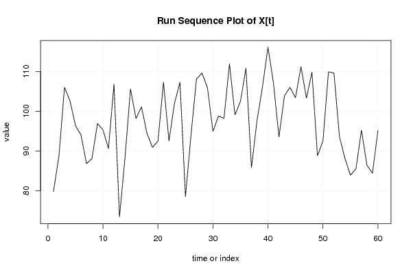
| Dataseries X: | |||||||||||||||||||||||||||||||||||||||||||||||||||||||||||||||||
79,8 88,8 106 102,6 96,4 94 86,8 88,1 96,9 95,3 90,6 106,8 73,4 88,2 105,6 98,2 101,1 94,4 90,9 92,5 107,3 92,5 102 107,3 78,5 93,9 108,1 109,6 105,9 94,9 98,8 98,2 111,9 99,1 102,5 110,8 85,8 97,6 106,1 116,1 107,1 93,5 103,9 106 103,4 111,2 103,3 109,8 88,8 92,5 109,9 109,6 93,6 88,1 83,9 85,5 95,2 86,4 84,4 95,2 | |||||||||||||||||||||||||||||||||||||||||||||||||||||||||||||||||
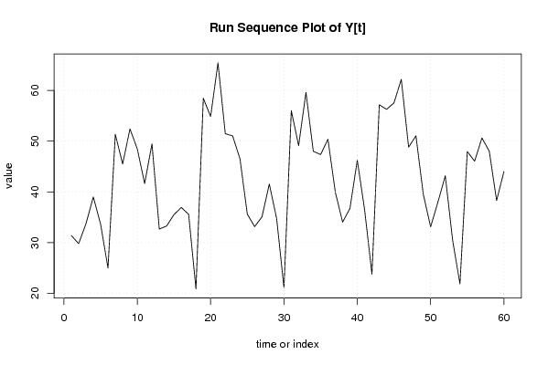
| Dataseries Y: | |||||||||||||||||||||||||||||||||||||||||||||||||||||||||||||||||
31.394 29.799 33.728 39.010 33.598 24.992 51.347 45.498 52.413 48.461 41.647 49.471 32.666 33.283 35.532 36.928 35.572 20.870 58.453 54.854 65.425 51.469 51.035 46.526 35.619 33.153 35.078 41.552 34.752 21.108 56.020 49.126 59.604 47.997 47.363 50.380 39.967 34.045 36.748 46.234 36.464 23.772 57.165 56.276 57.547 62.183 48.820 51.052 39.540 33.113 38.010 43.175 30.501 21.862 47.942 46.055 50.633 48.020 38.298 44.009 | |||||||||||||||||||||||||||||||||||||||||||||||||||||||||||||||||
Tables (Output of Computation) | |||||||||||||||||||||||||||||||||||||||||||||||||||||||||||||||||
| |||||||||||||||||||||||||||||||||||||||||||||||||||||||||||||||||
Figures (Output of Computation) | |||||||||||||||||||||||||||||||||||||||||||||||||||||||||||||||||
Input Parameters & R Code | |||||||||||||||||||||||||||||||||||||||||||||||||||||||||||||||||
| Parameters (Session): | |||||||||||||||||||||||||||||||||||||||||||||||||||||||||||||||||
| par1 = 0 ; par2 = 36 ; | |||||||||||||||||||||||||||||||||||||||||||||||||||||||||||||||||
| Parameters (R input): | |||||||||||||||||||||||||||||||||||||||||||||||||||||||||||||||||
| par1 = 0 ; par2 = 36 ; | |||||||||||||||||||||||||||||||||||||||||||||||||||||||||||||||||
| R code (references can be found in the software module): | |||||||||||||||||||||||||||||||||||||||||||||||||||||||||||||||||
par1 <- as.numeric(par1) | |||||||||||||||||||||||||||||||||||||||||||||||||||||||||||||||||