Free Statistics
of Irreproducible Research!
Description of Statistical Computation | |||||||||||||||||||||||||||||||||||||||||||||||||||||||||||||||||
|---|---|---|---|---|---|---|---|---|---|---|---|---|---|---|---|---|---|---|---|---|---|---|---|---|---|---|---|---|---|---|---|---|---|---|---|---|---|---|---|---|---|---|---|---|---|---|---|---|---|---|---|---|---|---|---|---|---|---|---|---|---|---|---|---|---|
| Author's title | |||||||||||||||||||||||||||||||||||||||||||||||||||||||||||||||||
| Author | *The author of this computation has been verified* | ||||||||||||||||||||||||||||||||||||||||||||||||||||||||||||||||
| R Software Module | rwasp_edabi.wasp | ||||||||||||||||||||||||||||||||||||||||||||||||||||||||||||||||
| Title produced by software | Bivariate Explorative Data Analysis | ||||||||||||||||||||||||||||||||||||||||||||||||||||||||||||||||
| Date of computation | Thu, 29 Oct 2009 05:36:59 -0600 | ||||||||||||||||||||||||||||||||||||||||||||||||||||||||||||||||
| Cite this page as follows | Statistical Computations at FreeStatistics.org, Office for Research Development and Education, URL https://freestatistics.org/blog/index.php?v=date/2009/Oct/29/t1256816331slqxu1llucho2uu.htm/, Retrieved Tue, 01 Jul 2025 03:21:33 +0000 | ||||||||||||||||||||||||||||||||||||||||||||||||||||||||||||||||
| Statistical Computations at FreeStatistics.org, Office for Research Development and Education, URL https://freestatistics.org/blog/index.php?pk=51921, Retrieved Tue, 01 Jul 2025 03:21:33 +0000 | |||||||||||||||||||||||||||||||||||||||||||||||||||||||||||||||||
| QR Codes: | |||||||||||||||||||||||||||||||||||||||||||||||||||||||||||||||||
|
| |||||||||||||||||||||||||||||||||||||||||||||||||||||||||||||||||
| Original text written by user: | |||||||||||||||||||||||||||||||||||||||||||||||||||||||||||||||||
| IsPrivate? | No (this computation is public) | ||||||||||||||||||||||||||||||||||||||||||||||||||||||||||||||||
| User-defined keywords | |||||||||||||||||||||||||||||||||||||||||||||||||||||||||||||||||
| Estimated Impact | 277 | ||||||||||||||||||||||||||||||||||||||||||||||||||||||||||||||||
Tree of Dependent Computations | |||||||||||||||||||||||||||||||||||||||||||||||||||||||||||||||||
| Family? (F = Feedback message, R = changed R code, M = changed R Module, P = changed Parameters, D = changed Data) | |||||||||||||||||||||||||||||||||||||||||||||||||||||||||||||||||
| - [Bivariate Data Series] [Bivariate dataset] [2008-01-05 23:51:08] [74be16979710d4c4e7c6647856088456] - RMPD [Bivariate Explorative Data Analysis] [WS4 Bivariate EDA...] [2009-10-27 17:41:15] [1d635fe1113b56bab3f378c464a289bc] - D [Bivariate Explorative Data Analysis] [WS304] [2009-10-29 11:36:59] [71c065898bd1c08eef04509b4bcee039] [Current] - D [Bivariate Explorative Data Analysis] [WS305] [2009-10-29 11:44:40] [4a2be4899cba879e4eea9daa25281df8] - RMPD [Trivariate Scatterplots] [Workshop 5.1] [2009-11-11 19:06:58] [4a2be4899cba879e4eea9daa25281df8] - RMPD [Bivariate Explorative Data Analysis] [Workshop 5.3] [2009-11-11 19:18:19] [4a2be4899cba879e4eea9daa25281df8] - RMPD [Bivariate Explorative Data Analysis] [Workshop 5.4] [2009-11-11 19:21:51] [4a2be4899cba879e4eea9daa25281df8] - RMPD [Bivariate Explorative Data Analysis] [Workshop 5.5] [2009-11-11 19:33:35] [4a2be4899cba879e4eea9daa25281df8] - RMPD [Pearson Correlation] [Workshop 5.6] [2009-11-11 19:36:06] [4a2be4899cba879e4eea9daa25281df8] - RMPD [Partial Correlation] [workshop 5.2] [2009-11-11 19:10:03] [4a2be4899cba879e4eea9daa25281df8] | |||||||||||||||||||||||||||||||||||||||||||||||||||||||||||||||||
| Feedback Forum | |||||||||||||||||||||||||||||||||||||||||||||||||||||||||||||||||
Post a new message | |||||||||||||||||||||||||||||||||||||||||||||||||||||||||||||||||
Dataset | |||||||||||||||||||||||||||||||||||||||||||||||||||||||||||||||||
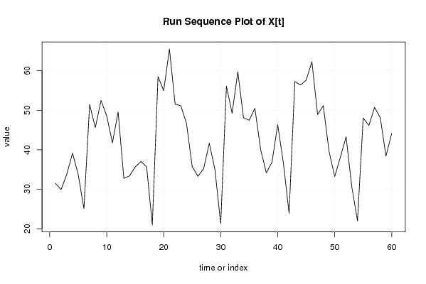
| Dataseries X: | |||||||||||||||||||||||||||||||||||||||||||||||||||||||||||||||||
31.481 29.896 33.842 39.120 33.702 25.094 51.442 45.594 52.518 48.564 41.745 49.585 32.747 33.379 35.645 37.034 35.681 20.972 58.552 54.955 65.540 51.570 51.145 46.641 35.704 33.253 35.193 41.668 34.865 21.210 56.126 49.231 59.723 48.103 47.472 50.497 40.059 34.149 36.860 46.356 36.577 23.872 57.276 56.389 57.657 62.300 48.929 51.168 39.636 33.213 38.127 43.291 30.600 21.956 48.033 46.148 50.736 48.114 38.390 44.112 | |||||||||||||||||||||||||||||||||||||||||||||||||||||||||||||||||
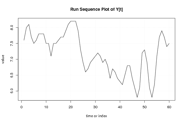
| Dataseries Y: | |||||||||||||||||||||||||||||||||||||||||||||||||||||||||||||||||
7,6 8 8,1 7,7 7,5 7,6 7,8 7,8 7,8 7,5 7,5 7,1 7,5 7,5 7,6 7,7 7,7 7,9 8,1 8,2 8,2 8,2 7,9 7,3 6,9 6,6 6,7 6,9 7 7,1 7,2 7,1 6,9 7 6,8 6,4 6,7 6,6 6,4 6,3 6,2 6,5 6,8 6,8 6,4 6,1 5,8 6,1 7,2 7,3 6,9 6,1 5,8 6,2 7,1 7,7 7,9 7,7 7,4 7,5 | |||||||||||||||||||||||||||||||||||||||||||||||||||||||||||||||||
Tables (Output of Computation) | |||||||||||||||||||||||||||||||||||||||||||||||||||||||||||||||||
| |||||||||||||||||||||||||||||||||||||||||||||||||||||||||||||||||
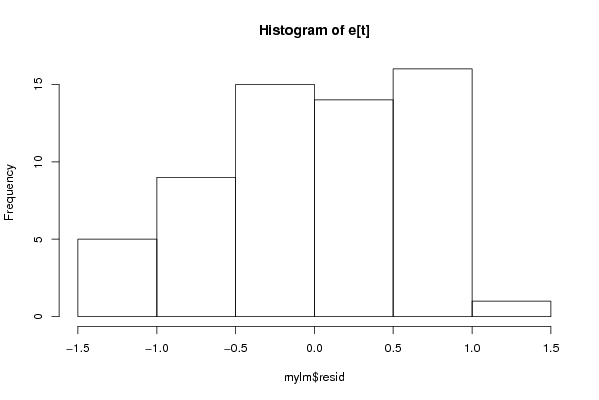
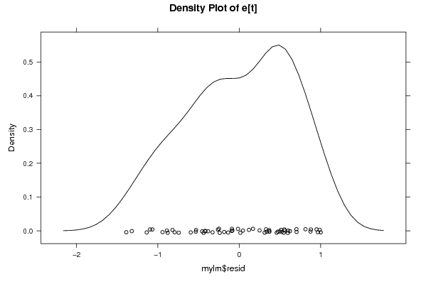
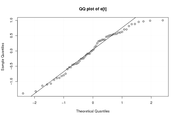
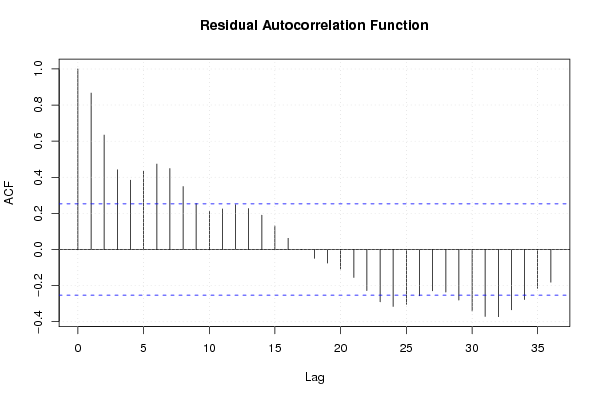
Figures (Output of Computation) | |||||||||||||||||||||||||||||||||||||||||||||||||||||||||||||||||
Input Parameters & R Code | |||||||||||||||||||||||||||||||||||||||||||||||||||||||||||||||||
| Parameters (Session): | |||||||||||||||||||||||||||||||||||||||||||||||||||||||||||||||||
| par1 = 0 ; par2 = 36 ; | |||||||||||||||||||||||||||||||||||||||||||||||||||||||||||||||||
| Parameters (R input): | |||||||||||||||||||||||||||||||||||||||||||||||||||||||||||||||||
| par1 = 0 ; par2 = 36 ; | |||||||||||||||||||||||||||||||||||||||||||||||||||||||||||||||||
| R code (references can be found in the software module): | |||||||||||||||||||||||||||||||||||||||||||||||||||||||||||||||||
par1 <- as.numeric(par1) | |||||||||||||||||||||||||||||||||||||||||||||||||||||||||||||||||