Free Statistics
of Irreproducible Research!
Description of Statistical Computation | |||||||||||||||||||||
|---|---|---|---|---|---|---|---|---|---|---|---|---|---|---|---|---|---|---|---|---|---|
| Author's title | |||||||||||||||||||||
| Author | *The author of this computation has been verified* | ||||||||||||||||||||
| R Software Module | rwasp_meanplot.wasp | ||||||||||||||||||||
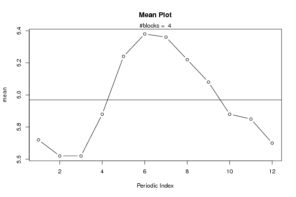
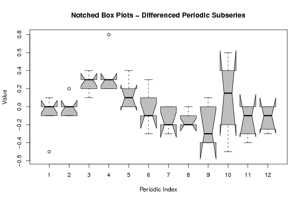
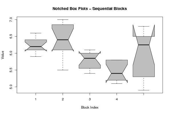
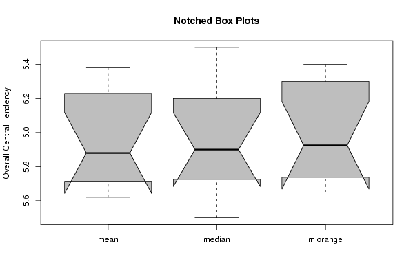
| Title produced by software | Mean Plot | ||||||||||||||||||||
| Date of computation | Wed, 11 Nov 2009 11:43:20 -0700 | ||||||||||||||||||||
| Cite this page as follows | Statistical Computations at FreeStatistics.org, Office for Research Development and Education, URL https://freestatistics.org/blog/index.php?v=date/2009/Nov/11/t1257965042rbbb8mkejj3xnxh.htm/, Retrieved Fri, 26 Apr 2024 09:01:24 +0000 | ||||||||||||||||||||
| Statistical Computations at FreeStatistics.org, Office for Research Development and Education, URL https://freestatistics.org/blog/index.php?pk=55808, Retrieved Fri, 26 Apr 2024 09:01:24 +0000 | |||||||||||||||||||||
| QR Codes: | |||||||||||||||||||||
|
| |||||||||||||||||||||
| Original text written by user: | |||||||||||||||||||||
| IsPrivate? | No (this computation is public) | ||||||||||||||||||||
| User-defined keywords | |||||||||||||||||||||
| Estimated Impact | 134 | ||||||||||||||||||||
Tree of Dependent Computations | |||||||||||||||||||||
| Family? (F = Feedback message, R = changed R code, M = changed R Module, P = changed Parameters, D = changed Data) | |||||||||||||||||||||
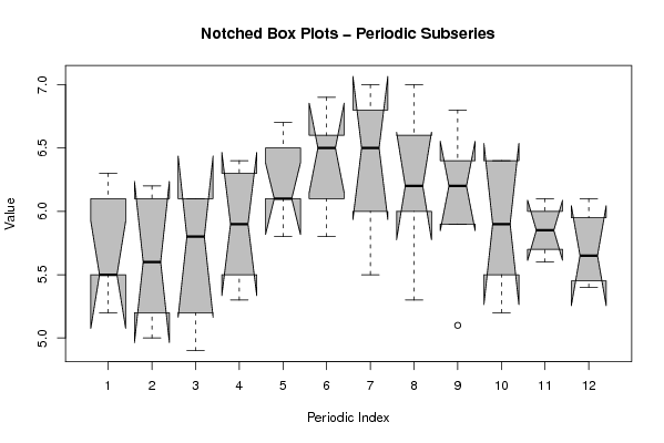
| - [Notched Boxplots] [3/11/2009] [2009-11-02 21:10:41] [b98453cac15ba1066b407e146608df68] - RMPD [Back to Back Histogram] [back-to-back werk...] [2009-11-11 17:58:46] [ba905ddf7cdf9ecb063c35348c4dab2e] - RM D [Mean Plot] [Mean plot] [2009-11-11 18:43:20] [244731fa3e7e6c85774b8c0902c58f85] [Current] | |||||||||||||||||||||
| Feedback Forum | |||||||||||||||||||||
Post a new message | |||||||||||||||||||||
Dataset | |||||||||||||||||||||
| Dataseries X: | |||||||||||||||||||||
6,3 6,2 6,1 6,3 6,5 6,6 6,5 6,2 6,2 5,9 6,1 6,1 6,1 6,1 6,1 6,4 6,7 6,9 7 7 6,8 6,4 5,9 5,5 5,5 5,6 5,8 5,9 6,1 6,1 6 6 5,9 5,5 5,6 5,4 5,2 5,2 5,2 5,5 5,8 5,8 5,5 5,3 5,1 5,2 5,8 5,8 5,5 5 4,9 5,3 6,1 6,5 6,8 6,6 6,4 6,4 | |||||||||||||||||||||
Tables (Output of Computation) | |||||||||||||||||||||
| |||||||||||||||||||||
Figures (Output of Computation) | |||||||||||||||||||||
Input Parameters & R Code | |||||||||||||||||||||
| Parameters (Session): | |||||||||||||||||||||
| par1 = grey ; par2 = grey ; par3 = TRUE ; par4 = Female ; par5 = Male ; | |||||||||||||||||||||
| Parameters (R input): | |||||||||||||||||||||
| par1 = 12 ; | |||||||||||||||||||||
| R code (references can be found in the software module): | |||||||||||||||||||||
par1 <- as.numeric(par1) | |||||||||||||||||||||