Free Statistics
of Irreproducible Research!
Description of Statistical Computation | |||||||||||||||||||||
|---|---|---|---|---|---|---|---|---|---|---|---|---|---|---|---|---|---|---|---|---|---|
| Author's title | |||||||||||||||||||||
| Author | *The author of this computation has been verified* | ||||||||||||||||||||
| R Software Module | rwasp_sdplot.wasp | ||||||||||||||||||||
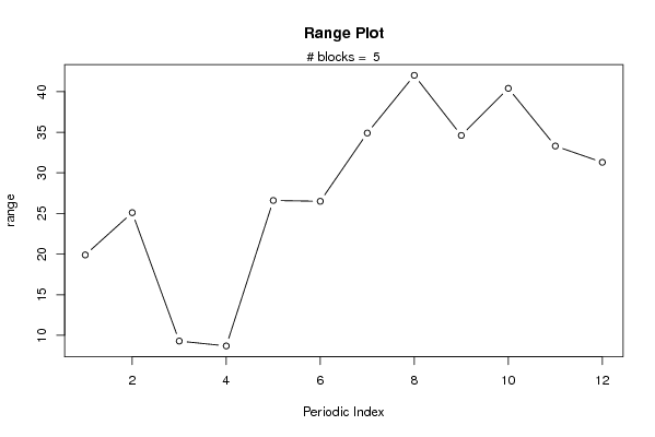
| Title produced by software | Standard Deviation Plot | ||||||||||||||||||||
| Date of computation | Tue, 10 Nov 2009 12:32:01 -0700 | ||||||||||||||||||||
| Cite this page as follows | Statistical Computations at FreeStatistics.org, Office for Research Development and Education, URL https://freestatistics.org/blog/index.php?v=date/2009/Nov/10/t1257881765pe99ul2pmvgm9ps.htm/, Retrieved Mon, 06 May 2024 09:21:04 +0000 | ||||||||||||||||||||
| Statistical Computations at FreeStatistics.org, Office for Research Development and Education, URL https://freestatistics.org/blog/index.php?pk=55357, Retrieved Mon, 06 May 2024 09:21:04 +0000 | |||||||||||||||||||||
| QR Codes: | |||||||||||||||||||||
|
| |||||||||||||||||||||
| Original text written by user: | |||||||||||||||||||||
| IsPrivate? | No (this computation is public) | ||||||||||||||||||||
| User-defined keywords | |||||||||||||||||||||
| Estimated Impact | 115 | ||||||||||||||||||||
Tree of Dependent Computations | |||||||||||||||||||||
| Family? (F = Feedback message, R = changed R code, M = changed R Module, P = changed Parameters, D = changed Data) | |||||||||||||||||||||
| - [Bivariate Explorative Data Analysis] [3/11/2009] [2009-11-02 22:01:32] [b98453cac15ba1066b407e146608df68] - RMPD [Standard Deviation Plot] [] [2009-11-10 19:32:01] [8551abdd6804649d94d88b1829ac2b1a] [Current] | |||||||||||||||||||||
| Feedback Forum | |||||||||||||||||||||
Post a new message | |||||||||||||||||||||
Dataset | |||||||||||||||||||||
| Dataseries X: | |||||||||||||||||||||
110,5 110,8 104,2 88,9 89,8 90 93,9 91,3 87,8 99,7 73,5 79,2 96,9 95,2 95,6 89,7 92,8 88 101,1 92,7 95,8 103,8 81,8 87,1 105,9 108,1 102,6 93,7 103,5 100,6 113,3 102,4 102,1 106,9 87,3 93,1 109,1 120,3 104,9 92,6 109,8 111,4 117,9 121,6 117,8 124,2 106,8 102,7 116,8 113,6 96,1 85 83,2 84,9 83 79,6 83,2 83,8 82,8 71,4 | |||||||||||||||||||||
Tables (Output of Computation) | |||||||||||||||||||||
| |||||||||||||||||||||
Figures (Output of Computation) | |||||||||||||||||||||
Input Parameters & R Code | |||||||||||||||||||||
| Parameters (Session): | |||||||||||||||||||||
| par1 = 0 ; par2 = 36 ; | |||||||||||||||||||||
| Parameters (R input): | |||||||||||||||||||||
| par1 = 12 ; | |||||||||||||||||||||
| R code (references can be found in the software module): | |||||||||||||||||||||
par1 <- as.numeric(par1) | |||||||||||||||||||||