Free Statistics
of Irreproducible Research!
Description of Statistical Computation | |||||||||||||||||||||
|---|---|---|---|---|---|---|---|---|---|---|---|---|---|---|---|---|---|---|---|---|---|
| Author's title | |||||||||||||||||||||
| Author | *The author of this computation has been verified* | ||||||||||||||||||||
| R Software Module | rwasp_meanplot.wasp | ||||||||||||||||||||
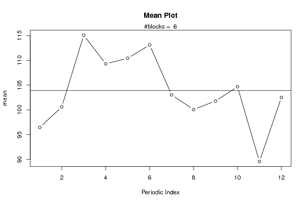
| Title produced by software | Mean Plot | ||||||||||||||||||||
| Date of computation | Tue, 10 Nov 2009 07:28:39 -0700 | ||||||||||||||||||||
| Cite this page as follows | Statistical Computations at FreeStatistics.org, Office for Research Development and Education, URL https://freestatistics.org/blog/index.php?v=date/2009/Nov/10/t1257863455wxt58a7lr6n9rn8.htm/, Retrieved Mon, 06 May 2024 10:07:51 +0000 | ||||||||||||||||||||
| Statistical Computations at FreeStatistics.org, Office for Research Development and Education, URL https://freestatistics.org/blog/index.php?pk=55249, Retrieved Mon, 06 May 2024 10:07:51 +0000 | |||||||||||||||||||||
| QR Codes: | |||||||||||||||||||||
|
| |||||||||||||||||||||
| Original text written by user: | |||||||||||||||||||||
| IsPrivate? | No (this computation is public) | ||||||||||||||||||||
| User-defined keywords | |||||||||||||||||||||
| Estimated Impact | 143 | ||||||||||||||||||||
Tree of Dependent Computations | |||||||||||||||||||||
| Family? (F = Feedback message, R = changed R code, M = changed R Module, P = changed Parameters, D = changed Data) | |||||||||||||||||||||
| - [Mean Plot] [3/11/2009] [2009-11-02 22:07:54] [b98453cac15ba1066b407e146608df68] - PD [Mean Plot] [ws2] [2009-11-10 14:28:39] [94ba0ef70f5b330d175ff4daa1c9cd40] [Current] - PD [Mean Plot] [ws2] [2009-11-12 14:14:18] [ca30429b07824e7c5d48293114d35d71] | |||||||||||||||||||||
| Feedback Forum | |||||||||||||||||||||
Post a new message | |||||||||||||||||||||
Dataset | |||||||||||||||||||||
| Dataseries X: | |||||||||||||||||||||
100.00 108.16 114.02 102.19 110.37 96.86 94.19 99.52 94.06 97.55 78.15 81.24 92.36 96.06 114.05 110.66 104.92 90.00 95.70 86.03 84.85 100.04 80.92 74.07 77.30 97.23 90.76 100.56 92.01 99.24 105.87 90.99 93.31 91.17 77.33 91.13 85.01 83.90 104.86 110.90 95.44 111.62 108.89 96.18 101.97 99.12 86.78 118.42 118.74 106.53 134.78 104.68 105.30 139.41 103.61 99.78 103.46 120.06 96.71 107.13 105.36 111.69 132.05 126.80 154.48 141.56 109.95 127.90 133.09 120.08 117.56 143.04 | |||||||||||||||||||||
Tables (Output of Computation) | |||||||||||||||||||||
| |||||||||||||||||||||
Figures (Output of Computation) | |||||||||||||||||||||
Input Parameters & R Code | |||||||||||||||||||||
| Parameters (Session): | |||||||||||||||||||||
| par1 = red ; par2 = blue ; par3 = TRUE ; par4 = BV ; par5 = BN ; | |||||||||||||||||||||
| Parameters (R input): | |||||||||||||||||||||
| par1 = 12 ; | |||||||||||||||||||||
| R code (references can be found in the software module): | |||||||||||||||||||||
par1 <- as.numeric(par1) | |||||||||||||||||||||