Free Statistics
of Irreproducible Research!
Description of Statistical Computation | |||||||||||||||||||||
|---|---|---|---|---|---|---|---|---|---|---|---|---|---|---|---|---|---|---|---|---|---|
| Author's title | |||||||||||||||||||||
| Author | *The author of this computation has been verified* | ||||||||||||||||||||
| R Software Module | rwasp_meanplot.wasp | ||||||||||||||||||||
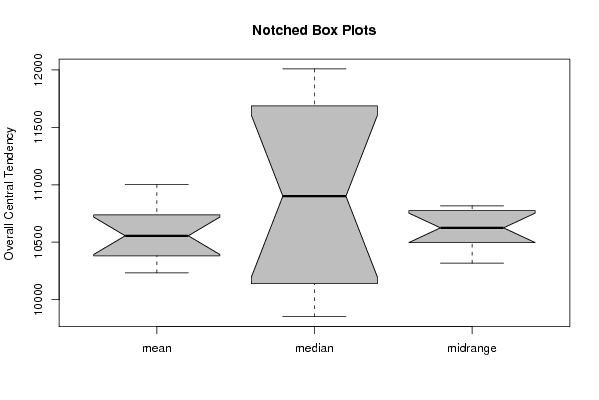
| Title produced by software | Mean Plot | ||||||||||||||||||||
| Date of computation | Tue, 10 Nov 2009 03:57:55 -0700 | ||||||||||||||||||||
| Cite this page as follows | Statistical Computations at FreeStatistics.org, Office for Research Development and Education, URL https://freestatistics.org/blog/index.php?v=date/2009/Nov/10/t1257850833ioo9d4tg2w257lr.htm/, Retrieved Sun, 05 May 2024 22:26:12 +0000 | ||||||||||||||||||||
| Statistical Computations at FreeStatistics.org, Office for Research Development and Education, URL https://freestatistics.org/blog/index.php?pk=55161, Retrieved Sun, 05 May 2024 22:26:12 +0000 | |||||||||||||||||||||
| QR Codes: | |||||||||||||||||||||
|
| |||||||||||||||||||||
| Original text written by user: | |||||||||||||||||||||
| IsPrivate? | No (this computation is public) | ||||||||||||||||||||
| User-defined keywords | |||||||||||||||||||||
| Estimated Impact | 139 | ||||||||||||||||||||
Tree of Dependent Computations | |||||||||||||||||||||
| Family? (F = Feedback message, R = changed R code, M = changed R Module, P = changed Parameters, D = changed Data) | |||||||||||||||||||||
| - [Mean Plot] [3/11/2009] [2009-11-02 22:07:54] [b98453cac15ba1066b407e146608df68] - D [Mean Plot] [] [2009-11-10 10:57:55] [90c9838c596c9c0a7d0d4c412ffe5b98] [Current] | |||||||||||||||||||||
| Feedback Forum | |||||||||||||||||||||
Post a new message | |||||||||||||||||||||
Dataset | |||||||||||||||||||||
| Dataseries X: | |||||||||||||||||||||
6802.96 7132.68 7073.29 7264.5 7105.33 7218.71 7225.72 7354.25 7745.46 8070.26 8366.33 8667.51 8854.34 9218.1 9332.9 9358.31 9248.66 9401.2 9652.04 9957.38 10110.63 10169.26 10343.78 10750.21 11337.5 11786.96 12083.04 12007.74 11745.93 11051.51 11445.9 11924.88 12247.63 12690.91 12910.7 13202.12 13654.67 13862.82 13523.93 14211.17 14510.35 14289.23 14111.82 13086.59 13351.54 13747.69 12855.61 12926.93 12121.95 11731.65 11639.51 12163.78 12029.53 11234.18 9852.13 9709.04 9332.75 7108.6 6691.49 6143.05 | |||||||||||||||||||||
Tables (Output of Computation) | |||||||||||||||||||||
| |||||||||||||||||||||
Figures (Output of Computation) | |||||||||||||||||||||
Input Parameters & R Code | |||||||||||||||||||||
| Parameters (Session): | |||||||||||||||||||||
| Parameters (R input): | |||||||||||||||||||||
| par1 = 12 ; | |||||||||||||||||||||
| R code (references can be found in the software module): | |||||||||||||||||||||
par1 <- as.numeric(par1) | |||||||||||||||||||||