Free Statistics
of Irreproducible Research!
Description of Statistical Computation | |||||||||||||||||||||
|---|---|---|---|---|---|---|---|---|---|---|---|---|---|---|---|---|---|---|---|---|---|
| Author's title | |||||||||||||||||||||
| Author | *The author of this computation has been verified* | ||||||||||||||||||||
| R Software Module | rwasp_cloud.wasp | ||||||||||||||||||||
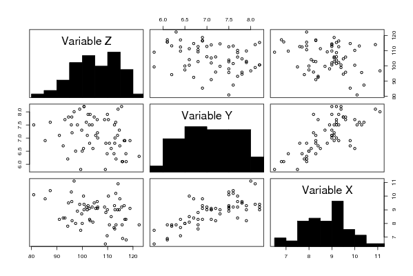
| Title produced by software | Trivariate Scatterplots | ||||||||||||||||||||
| Date of computation | Sat, 07 Nov 2009 03:22:32 -0700 | ||||||||||||||||||||
| Cite this page as follows | Statistical Computations at FreeStatistics.org, Office for Research Development and Education, URL https://freestatistics.org/blog/index.php?v=date/2009/Nov/07/t1257589553lpl14bjdk6hlq1f.htm/, Retrieved Mon, 06 May 2024 18:46:53 +0000 | ||||||||||||||||||||
| Statistical Computations at FreeStatistics.org, Office for Research Development and Education, URL https://freestatistics.org/blog/index.php?pk=54380, Retrieved Mon, 06 May 2024 18:46:53 +0000 | |||||||||||||||||||||
| QR Codes: | |||||||||||||||||||||
|
| |||||||||||||||||||||
| Original text written by user: | |||||||||||||||||||||
| IsPrivate? | No (this computation is public) | ||||||||||||||||||||
| User-defined keywords | |||||||||||||||||||||
| Estimated Impact | 182 | ||||||||||||||||||||
Tree of Dependent Computations | |||||||||||||||||||||
| Family? (F = Feedback message, R = changed R code, M = changed R Module, P = changed Parameters, D = changed Data) | |||||||||||||||||||||
| - [Bivariate Data Series] [Bivariate dataset] [2008-01-05 23:51:08] [74be16979710d4c4e7c6647856088456] - RMPD [Bivariate Explorative Data Analysis] [Bivariate EDA par...] [2009-10-21 15:12:14] [2f74b736c031245eb7b9a6567f4b8492] - D [Bivariate Explorative Data Analysis] [Ln] [2009-10-27 16:19:13] [2f74b736c031245eb7b9a6567f4b8492] - RMPD [Partial Correlation] [Partial Correlati...] [2009-10-28 16:14:27] [2f74b736c031245eb7b9a6567f4b8492] - RMP [Trivariate Scatterplots] [WS 5 Review ] [2009-11-07 10:22:32] [eba9f01697e64705b70041e6f338cb22] [Current] | |||||||||||||||||||||
| Feedback Forum | |||||||||||||||||||||
Post a new message | |||||||||||||||||||||
Dataset | |||||||||||||||||||||
| Dataseries X: | |||||||||||||||||||||
9.3 8.3 8 8.5 10.4 11.1 10.9 10 9.2 9.2 9.5 9.6 9.5 9.1 8.9 9 10.1 10.3 10.2 9.6 9.2 9.3 9.4 9.4 9.2 9 9 9 9.8 10 9.8 9.3 9 9 9.1 9.1 9.1 9.2 8.8 8.3 8.4 8.1 7.7 7.9 7.9 8 7.9 7.6 7.1 6.8 6.5 6.9 8.2 8.7 8.3 7.9 7.5 7.8 8.3 8.4 8.2 | |||||||||||||||||||||
| Dataseries Y: | |||||||||||||||||||||
7.5 6.8 6.5 6.6 7.6 8 8.1 7.7 7.5 7.6 7.8 7.8 7.8 7.5 7.5 7.1 7.5 7.5 7.6 7.7 7.7 7.9 8.1 8.2 8.2 8.2 7.9 7.3 6.9 6.6 6.7 6.9 7 7.1 7.2 7.1 6.9 7 6.8 6.4 6.7 6.6 6.4 6.3 6.2 6.5 6.8 6.8 6.4 6.1 5.8 6.1 7.2 7.3 6.9 6.1 5.8 6.2 7.1 7.7 7.9 | |||||||||||||||||||||
| Dataseries Z: | |||||||||||||||||||||
112.7 102.9 97.4 111.4 87.4 96.8 114.1 110.3 103.9 101.6 94.6 95.9 104.7 102.8 98.1 113.9 80.9 95.7 113.2 105.9 108.8 102.3 99 100.7 115.5 100.7 109.9 114.6 85.4 100.5 114.8 116.5 112.9 102 106 105.3 118.8 106.1 109.3 117.2 92.5 104.2 112.5 122.4 113.3 100 110.7 112.8 109.8 117.3 109.1 115.9 96 99.8 116.8 115.7 99.4 94.3 91 93.2 103.1 | |||||||||||||||||||||
Tables (Output of Computation) | |||||||||||||||||||||
| |||||||||||||||||||||
Figures (Output of Computation) | |||||||||||||||||||||
Input Parameters & R Code | |||||||||||||||||||||
| Parameters (Session): | |||||||||||||||||||||
| par1 = 50 ; par2 = 50 ; par3 = Y ; par4 = Y ; par5 = Variable X ; par6 = Variable Y ; par7 = Variable Z ; | |||||||||||||||||||||
| Parameters (R input): | |||||||||||||||||||||
| par1 = 50 ; par2 = 50 ; par3 = Y ; par4 = Y ; par5 = Variable X ; par6 = Variable Y ; par7 = Variable Z ; | |||||||||||||||||||||
| R code (references can be found in the software module): | |||||||||||||||||||||
x <- array(x,dim=c(length(x),1)) | |||||||||||||||||||||