Free Statistics
of Irreproducible Research!
Description of Statistical Computation | |||||||||||||||||||||||||||||||||||||||||||||||||||||||||||||||||
|---|---|---|---|---|---|---|---|---|---|---|---|---|---|---|---|---|---|---|---|---|---|---|---|---|---|---|---|---|---|---|---|---|---|---|---|---|---|---|---|---|---|---|---|---|---|---|---|---|---|---|---|---|---|---|---|---|---|---|---|---|---|---|---|---|---|
| Author's title | |||||||||||||||||||||||||||||||||||||||||||||||||||||||||||||||||
| Author | *The author of this computation has been verified* | ||||||||||||||||||||||||||||||||||||||||||||||||||||||||||||||||
| R Software Module | rwasp_edabi.wasp | ||||||||||||||||||||||||||||||||||||||||||||||||||||||||||||||||
| Title produced by software | Bivariate Explorative Data Analysis | ||||||||||||||||||||||||||||||||||||||||||||||||||||||||||||||||
| Date of computation | Wed, 21 Oct 2009 09:12:14 -0600 | ||||||||||||||||||||||||||||||||||||||||||||||||||||||||||||||||
| Cite this page as follows | Statistical Computations at FreeStatistics.org, Office for Research Development and Education, URL https://freestatistics.org/blog/index.php?v=date/2009/Oct/21/t1256137999jbj1pwhfcb4jzr5.htm/, Retrieved Sun, 13 Jul 2025 02:59:01 +0000 | ||||||||||||||||||||||||||||||||||||||||||||||||||||||||||||||||
| Statistical Computations at FreeStatistics.org, Office for Research Development and Education, URL https://freestatistics.org/blog/index.php?pk=49404, Retrieved Sun, 13 Jul 2025 02:59:01 +0000 | |||||||||||||||||||||||||||||||||||||||||||||||||||||||||||||||||
| QR Codes: | |||||||||||||||||||||||||||||||||||||||||||||||||||||||||||||||||
|
| |||||||||||||||||||||||||||||||||||||||||||||||||||||||||||||||||
| Original text written by user: | |||||||||||||||||||||||||||||||||||||||||||||||||||||||||||||||||
| IsPrivate? | No (this computation is public) | ||||||||||||||||||||||||||||||||||||||||||||||||||||||||||||||||
| User-defined keywords | |||||||||||||||||||||||||||||||||||||||||||||||||||||||||||||||||
| Estimated Impact | 315 | ||||||||||||||||||||||||||||||||||||||||||||||||||||||||||||||||
Tree of Dependent Computations | |||||||||||||||||||||||||||||||||||||||||||||||||||||||||||||||||
| Family? (F = Feedback message, R = changed R code, M = changed R Module, P = changed Parameters, D = changed Data) | |||||||||||||||||||||||||||||||||||||||||||||||||||||||||||||||||
| - [Bivariate Data Series] [Bivariate dataset] [2008-01-05 23:51:08] [74be16979710d4c4e7c6647856088456] - RMPD [Bivariate Explorative Data Analysis] [Bivariate EDA par...] [2009-10-21 15:12:14] [eeda0e496238f8886c14dbbeff6ff613] [Current] - D [Bivariate Explorative Data Analysis] [Ln] [2009-10-27 16:19:13] [2f74b736c031245eb7b9a6567f4b8492] - RMP [Kendall tau Rank Correlation] [Kendall tau Rank ...] [2009-10-28 15:55:47] [2f74b736c031245eb7b9a6567f4b8492] - RMPD [Trivariate Scatterplots] [Trivariate Scatte...] [2009-10-28 16:11:45] [2f74b736c031245eb7b9a6567f4b8492] - RMPD [Partial Correlation] [Partial Correlati...] [2009-10-28 16:14:27] [2f74b736c031245eb7b9a6567f4b8492] - RMP [Trivariate Scatterplots] [WS 5 Review ] [2009-11-07 10:22:32] [83058a88a37d754675a5cd22dab372fc] - D [Bivariate Explorative Data Analysis] [Bivariate EDA WS5] [2009-10-28 16:21:27] [2f74b736c031245eb7b9a6567f4b8492] - D [Bivariate Explorative Data Analysis] [Bivariate EDA WS5] [2009-10-28 16:26:59] [2f74b736c031245eb7b9a6567f4b8492] - D [Bivariate Explorative Data Analysis] [Bivariate EDA WS5 ] [2009-10-28 16:30:59] [2f74b736c031245eb7b9a6567f4b8492] - M D [Bivariate Explorative Data Analysis] [Bivariate EDA ] [2009-11-09 08:25:54] [2f74b736c031245eb7b9a6567f4b8492] - RMPD [Mean Plot] [Mean plot] [2009-11-09 08:33:49] [2f74b736c031245eb7b9a6567f4b8492] - RMPD [Standard Deviation Plot] [Standard Deviatio...] [2009-11-09 08:38:22] [2f74b736c031245eb7b9a6567f4b8492] | |||||||||||||||||||||||||||||||||||||||||||||||||||||||||||||||||
| Feedback Forum | |||||||||||||||||||||||||||||||||||||||||||||||||||||||||||||||||
Post a new message | |||||||||||||||||||||||||||||||||||||||||||||||||||||||||||||||||
Dataset | |||||||||||||||||||||||||||||||||||||||||||||||||||||||||||||||||
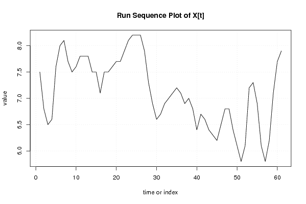
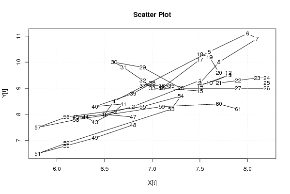
| Dataseries X: | |||||||||||||||||||||||||||||||||||||||||||||||||||||||||||||||||
7,5 6,8 6,5 6,6 7,6 8 8,1 7,7 7,5 7,6 7,8 7,8 7,8 7,5 7,5 7,1 7,5 7,5 7,6 7,7 7,7 7,9 8,1 8,2 8,2 8,2 7,9 7,3 6,9 6,6 6,7 6,9 7 7,1 7,2 7,1 6,9 7 6,8 6,4 6,7 6,6 6,4 6,3 6,2 6,5 6,8 6,8 6,4 6,1 5,8 6,1 7,2 7,3 6,9 6,1 5,8 6,2 7,1 7,7 7,9 | |||||||||||||||||||||||||||||||||||||||||||||||||||||||||||||||||
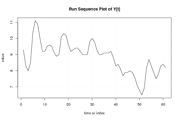
| Dataseries Y: | |||||||||||||||||||||||||||||||||||||||||||||||||||||||||||||||||
9,3 8,3 8 8,5 10,4 11,1 10,9 10 9,2 9,2 9,5 9,6 9,5 9,1 8,9 9 10,1 10,3 10,2 9,6 9,2 9,3 9,4 9,4 9,2 9 9 9 9,8 10 9,8 9,3 9 9 9,1 9,1 9,1 9,2 8,8 8,3 8,4 8,1 7,7 7,9 7,9 8 7,9 7,6 7,1 6,8 6,5 6,9 8,2 8,7 8,3 7,9 7,5 7,8 8,3 8,4 8,2 | |||||||||||||||||||||||||||||||||||||||||||||||||||||||||||||||||
Tables (Output of Computation) | |||||||||||||||||||||||||||||||||||||||||||||||||||||||||||||||||
| |||||||||||||||||||||||||||||||||||||||||||||||||||||||||||||||||
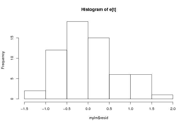
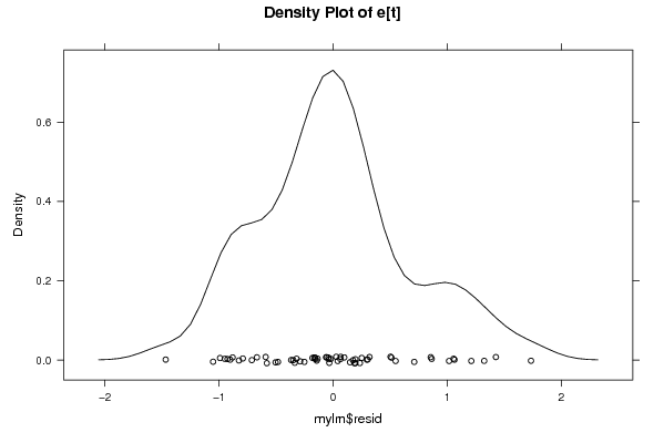
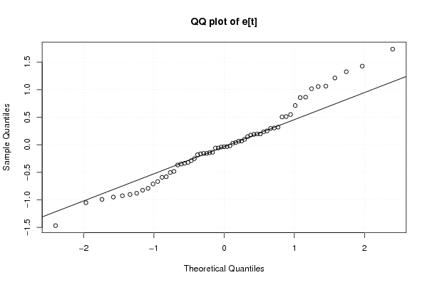
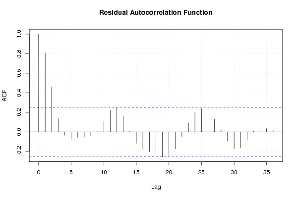
Figures (Output of Computation) | |||||||||||||||||||||||||||||||||||||||||||||||||||||||||||||||||
Input Parameters & R Code | |||||||||||||||||||||||||||||||||||||||||||||||||||||||||||||||||
| Parameters (Session): | |||||||||||||||||||||||||||||||||||||||||||||||||||||||||||||||||
| par1 = 0 ; par2 = 36 ; | |||||||||||||||||||||||||||||||||||||||||||||||||||||||||||||||||
| Parameters (R input): | |||||||||||||||||||||||||||||||||||||||||||||||||||||||||||||||||
| par1 = 0 ; par2 = 36 ; | |||||||||||||||||||||||||||||||||||||||||||||||||||||||||||||||||
| R code (references can be found in the software module): | |||||||||||||||||||||||||||||||||||||||||||||||||||||||||||||||||
par1 <- as.numeric(par1) | |||||||||||||||||||||||||||||||||||||||||||||||||||||||||||||||||