Free Statistics
of Irreproducible Research!
Description of Statistical Computation | |||||||||||||||||||||
|---|---|---|---|---|---|---|---|---|---|---|---|---|---|---|---|---|---|---|---|---|---|
| Author's title | |||||||||||||||||||||
| Author | *The author of this computation has been verified* | ||||||||||||||||||||
| R Software Module | rwasp_meanplot.wasp | ||||||||||||||||||||
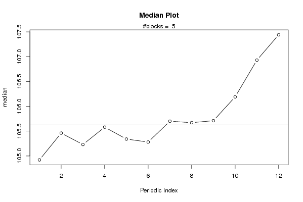
| Title produced by software | Mean Plot | ||||||||||||||||||||
| Date of computation | Tue, 15 Dec 2009 09:49:13 -0700 | ||||||||||||||||||||
| Cite this page as follows | Statistical Computations at FreeStatistics.org, Office for Research Development and Education, URL https://freestatistics.org/blog/index.php?v=date/2009/Dec/15/t12608958115ivd28smnghj487.htm/, Retrieved Wed, 08 May 2024 12:58:15 +0000 | ||||||||||||||||||||
| Statistical Computations at FreeStatistics.org, Office for Research Development and Education, URL https://freestatistics.org/blog/index.php?pk=68035, Retrieved Wed, 08 May 2024 12:58:15 +0000 | |||||||||||||||||||||
| QR Codes: | |||||||||||||||||||||
|
| |||||||||||||||||||||
| Original text written by user: | |||||||||||||||||||||
| IsPrivate? | No (this computation is public) | ||||||||||||||||||||
| User-defined keywords | |||||||||||||||||||||
| Estimated Impact | 100 | ||||||||||||||||||||
Tree of Dependent Computations | |||||||||||||||||||||
| Family? (F = Feedback message, R = changed R code, M = changed R Module, P = changed Parameters, D = changed Data) | |||||||||||||||||||||
| - [Mean Plot] [3/11/2009] [2009-11-02 22:07:54] [b98453cac15ba1066b407e146608df68] - R PD [Mean Plot] [mean plot] [2009-11-13 12:38:43] [3445d50c581a74ea3ff7b84cc82fcfeb] - D [Mean Plot] [] [2009-12-15 16:49:13] [c60887983b0820a525cba943a935572d] [Current] | |||||||||||||||||||||
| Feedback Forum | |||||||||||||||||||||
Post a new message | |||||||||||||||||||||
Dataset | |||||||||||||||||||||
| Dataseries X: | |||||||||||||||||||||
100.8 101.33 101.88 101.85 102.04 102.22 102.63 102.65 102.54 102.37 102.68 102.76 102.82 103.31 103.23 103.6 103.95 103.93 104.25 104.38 104.36 104.32 104.58 104.68 104.92 105.46 105.23 105.58 105.34 105.28 105.7 105.67 105.71 106.19 106.93 107.44 107.85 108.71 109.32 109.49 110.2 110.62 111.22 110.88 111.15 111.29 111.09 111.24 111.45 111.75 111.07 111.17 110.96 110.5 110.48 110.66 110.46 110.64 110.75 110.84 | |||||||||||||||||||||
Tables (Output of Computation) | |||||||||||||||||||||
| |||||||||||||||||||||
Figures (Output of Computation) | |||||||||||||||||||||
Input Parameters & R Code | |||||||||||||||||||||
| Parameters (Session): | |||||||||||||||||||||
| par1 = 12 ; | |||||||||||||||||||||
| Parameters (R input): | |||||||||||||||||||||
| par1 = 12 ; | |||||||||||||||||||||
| R code (references can be found in the software module): | |||||||||||||||||||||
par1 <- as.numeric(par1) | |||||||||||||||||||||