Repository of Reproducible Computations

Free Statistics

of Irreproducible Research!

Author's title

Author

*The author of this computation has been verified*

R Software Module

rwasp_autocorrelation.wasp

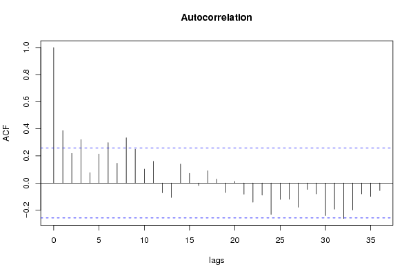
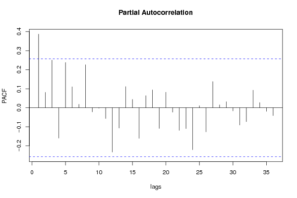
Title produced by software

(Partial) Autocorrelation Function

Date of computation

Fri, 11 Dec 2009 04:51:14 -0700

Cite this page as follows

Statistical Computations at FreeStatistics.org, Office for Research Development and Education, URL https://freestatistics.org/blog/index.php?v=date/2009/Dec/11/t12605323540xkyneklzidhojm.htm/, Retrieved Mon, 29 Apr 2024 03:25:23 +0000

Statistical Computations at FreeStatistics.org, Office for Research Development and Education, URL https://freestatistics.org/blog/index.php?pk=66034, Retrieved Mon, 29 Apr 2024 03:25:23 +0000

QR Codes:

Paste this QR Code to cite your computation.

Original text written by user:

IsPrivate?

No (this computation is public)

User-defined keywords

ACF2paper

Estimated Impact

172

Family? (F = Feedback message, R = changed R code, M = changed R Module, P = changed Parameters, D = changed Data)

-     [(Partial) Autocorrelation Function] [Partial autocorre...] [2008-12-09 20:18:51] [12d343c4448a5f9e527bb31caeac580b]
-   P   [(Partial) Autocorrelation Function] [Partial autocorre...] [2008-12-09 20:27:26] [12d343c4448a5f9e527bb31caeac580b]
-  MPD      [(Partial) Autocorrelation Function] [] [2009-12-11 11:51:14] [42ed2e0ab6f351a3dce7cf3f388e378d] [Current]
-   P         [(Partial) Autocorrelation Function] [] [2009-12-11 12:06:31] [cf890101a20378422561610e0d41fd9c] 
- R PD        [(Partial) Autocorrelation Function] [] [2010-12-21 12:03:44] [4f85667043e8913570b3eb8f368f82b2] 
- R PD        [(Partial) Autocorrelation Function] [] [2010-12-21 13:14:30] [4f85667043e8913570b3eb8f368f82b2] 
- R PD        [(Partial) Autocorrelation Function] [] [2010-12-21 19:24:48] [4f85667043e8913570b3eb8f368f82b2] 
- R PD        [(Partial) Autocorrelation Function] [] [2010-12-22 10:09:35] [4f85667043e8913570b3eb8f368f82b2] 

Feedback Forum

Post a new message

Dataseries X:

Download CSV

Histogram

Boxplots

Summary of computational transaction
Raw Input	view raw input (R code)
Raw Output	view raw output of R engine
Computing time	1 seconds
R Server	'Gwilym Jenkins' @ 72.249.127.135

\begin{tabular}{lllllllll}
\hline
Summary of computational transaction \tabularnewline
Raw Input & view raw input (R code)  \tabularnewline
Raw Output & view raw output of R engine  \tabularnewline
Computing time & 1 seconds \tabularnewline
R Server & 'Gwilym Jenkins' @ 72.249.127.135 \tabularnewline
\hline
\end{tabular}
%Source: https://freestatistics.org/blog/index.php?pk=66034&T=0

[TABLE]
[ROW][C]Summary of computational transaction[/C][/ROW]
[ROW][C]Raw Input[/C][C]view raw input (R code) [/C][/ROW]
[ROW][C]Raw Output[/C][C]view raw output of R engine [/C][/ROW]
[ROW][C]Computing time[/C][C]1 seconds[/C][/ROW]
[ROW][C]R Server[/C][C]'Gwilym Jenkins' @ 72.249.127.135[/C][/ROW]
[/TABLE]
Source: https://freestatistics.org/blog/index.php?pk=66034&T=0

Globally Unique Identifier (entire table): ba.freestatistics.org/blog/index.php?pk=66034&T=0

As an alternative you can also use a QR Code:

The GUIDs for individual cells are displayed in the table below:

Summary of computational transaction
Raw Input	view raw input (R code)
Raw Output	view raw output of R engine
Computing time	1 seconds
R Server	'Gwilym Jenkins' @ 72.249.127.135

Autocorrelation Function
Time lag k	ACF(k)	T-STAT	P-value
1	0.387107	2.9481	0.0023
2	0.218875	1.6669	0.050463
3	0.320872	2.4437	0.008801
4	0.076446	0.5822	0.281345
5	0.214129	1.6308	0.05418
6	0.298616	2.2742	0.013335
7	0.145952	1.1115	0.135462
8	0.333951	2.5433	0.006835
9	0.249593	1.9008	0.031148
10	0.10252	0.7808	0.219057
11	0.160311	1.2209	0.113534
12	-0.072619	-0.5531	0.291177
13	-0.106655	-0.8123	0.209981
14	0.139823	1.0649	0.145677
15	0.071749	0.5464	0.293435
16	-0.019071	-0.1452	0.442512
17	0.090929	0.6925	0.245694
18	0.029197	0.2224	0.412409
19	-0.070134	-0.5341	0.297649
20	0.011434	0.0871	0.465455
21	-0.082271	-0.6266	0.266703
22	-0.141426	-1.0771	0.142955
23	-0.089439	-0.6811	0.249244
24	-0.231911	-1.7662	0.041314
25	-0.121553	-0.9257	0.179213
26	-0.120291	-0.9161	0.181701
27	-0.178938	-1.3628	0.089114
28	-0.047274	-0.36	0.360068
29	-0.080777	-0.6152	0.270421
30	-0.240257	-1.8297	0.036215
31	-0.193563	-1.4741	0.072927
32	-0.261882	-1.9944	0.025406
33	-0.198104	-1.5087	0.0684
34	-0.080788	-0.6153	0.270393
35	-0.099017	-0.7541	0.226923
36	-0.055934	-0.426	0.335849

\begin{tabular}{lllllllll}
\hline
Autocorrelation Function \tabularnewline
Time lag k & ACF(k) & T-STAT & P-value \tabularnewline
1 & 0.387107 & 2.9481 & 0.0023 \tabularnewline
2 & 0.218875 & 1.6669 & 0.050463 \tabularnewline
3 & 0.320872 & 2.4437 & 0.008801 \tabularnewline
4 & 0.076446 & 0.5822 & 0.281345 \tabularnewline
5 & 0.214129 & 1.6308 & 0.05418 \tabularnewline
6 & 0.298616 & 2.2742 & 0.013335 \tabularnewline
7 & 0.145952 & 1.1115 & 0.135462 \tabularnewline
8 & 0.333951 & 2.5433 & 0.006835 \tabularnewline
9 & 0.249593 & 1.9008 & 0.031148 \tabularnewline
10 & 0.10252 & 0.7808 & 0.219057 \tabularnewline
11 & 0.160311 & 1.2209 & 0.113534 \tabularnewline
12 & -0.072619 & -0.5531 & 0.291177 \tabularnewline
13 & -0.106655 & -0.8123 & 0.209981 \tabularnewline
14 & 0.139823 & 1.0649 & 0.145677 \tabularnewline
15 & 0.071749 & 0.5464 & 0.293435 \tabularnewline
16 & -0.019071 & -0.1452 & 0.442512 \tabularnewline
17 & 0.090929 & 0.6925 & 0.245694 \tabularnewline
18 & 0.029197 & 0.2224 & 0.412409 \tabularnewline
19 & -0.070134 & -0.5341 & 0.297649 \tabularnewline
20 & 0.011434 & 0.0871 & 0.465455 \tabularnewline
21 & -0.082271 & -0.6266 & 0.266703 \tabularnewline
22 & -0.141426 & -1.0771 & 0.142955 \tabularnewline
23 & -0.089439 & -0.6811 & 0.249244 \tabularnewline
24 & -0.231911 & -1.7662 & 0.041314 \tabularnewline
25 & -0.121553 & -0.9257 & 0.179213 \tabularnewline
26 & -0.120291 & -0.9161 & 0.181701 \tabularnewline
27 & -0.178938 & -1.3628 & 0.089114 \tabularnewline
28 & -0.047274 & -0.36 & 0.360068 \tabularnewline
29 & -0.080777 & -0.6152 & 0.270421 \tabularnewline
30 & -0.240257 & -1.8297 & 0.036215 \tabularnewline
31 & -0.193563 & -1.4741 & 0.072927 \tabularnewline
32 & -0.261882 & -1.9944 & 0.025406 \tabularnewline
33 & -0.198104 & -1.5087 & 0.0684 \tabularnewline
34 & -0.080788 & -0.6153 & 0.270393 \tabularnewline
35 & -0.099017 & -0.7541 & 0.226923 \tabularnewline
36 & -0.055934 & -0.426 & 0.335849 \tabularnewline
\hline
\end{tabular}
%Source: https://freestatistics.org/blog/index.php?pk=66034&T=1

[TABLE]
[ROW][C]Autocorrelation Function[/C][/ROW]
[ROW][C]Time lag k[/C][C]ACF(k)[/C][C]T-STAT[/C][C]P-value[/C][/ROW]
[ROW][C]1[/C][C]0.387107[/C][C]2.9481[/C][C]0.0023[/C][/ROW]
[ROW][C]2[/C][C]0.218875[/C][C]1.6669[/C][C]0.050463[/C][/ROW]
[ROW][C]3[/C][C]0.320872[/C][C]2.4437[/C][C]0.008801[/C][/ROW]
[ROW][C]4[/C][C]0.076446[/C][C]0.5822[/C][C]0.281345[/C][/ROW]
[ROW][C]5[/C][C]0.214129[/C][C]1.6308[/C][C]0.05418[/C][/ROW]
[ROW][C]6[/C][C]0.298616[/C][C]2.2742[/C][C]0.013335[/C][/ROW]
[ROW][C]7[/C][C]0.145952[/C][C]1.1115[/C][C]0.135462[/C][/ROW]
[ROW][C]8[/C][C]0.333951[/C][C]2.5433[/C][C]0.006835[/C][/ROW]
[ROW][C]9[/C][C]0.249593[/C][C]1.9008[/C][C]0.031148[/C][/ROW]
[ROW][C]10[/C][C]0.10252[/C][C]0.7808[/C][C]0.219057[/C][/ROW]
[ROW][C]11[/C][C]0.160311[/C][C]1.2209[/C][C]0.113534[/C][/ROW]
[ROW][C]12[/C][C]-0.072619[/C][C]-0.5531[/C][C]0.291177[/C][/ROW]
[ROW][C]13[/C][C]-0.106655[/C][C]-0.8123[/C][C]0.209981[/C][/ROW]
[ROW][C]14[/C][C]0.139823[/C][C]1.0649[/C][C]0.145677[/C][/ROW]
[ROW][C]15[/C][C]0.071749[/C][C]0.5464[/C][C]0.293435[/C][/ROW]
[ROW][C]16[/C][C]-0.019071[/C][C]-0.1452[/C][C]0.442512[/C][/ROW]
[ROW][C]17[/C][C]0.090929[/C][C]0.6925[/C][C]0.245694[/C][/ROW]
[ROW][C]18[/C][C]0.029197[/C][C]0.2224[/C][C]0.412409[/C][/ROW]
[ROW][C]19[/C][C]-0.070134[/C][C]-0.5341[/C][C]0.297649[/C][/ROW]
[ROW][C]20[/C][C]0.011434[/C][C]0.0871[/C][C]0.465455[/C][/ROW]
[ROW][C]21[/C][C]-0.082271[/C][C]-0.6266[/C][C]0.266703[/C][/ROW]
[ROW][C]22[/C][C]-0.141426[/C][C]-1.0771[/C][C]0.142955[/C][/ROW]
[ROW][C]23[/C][C]-0.089439[/C][C]-0.6811[/C][C]0.249244[/C][/ROW]
[ROW][C]24[/C][C]-0.231911[/C][C]-1.7662[/C][C]0.041314[/C][/ROW]
[ROW][C]25[/C][C]-0.121553[/C][C]-0.9257[/C][C]0.179213[/C][/ROW]
[ROW][C]26[/C][C]-0.120291[/C][C]-0.9161[/C][C]0.181701[/C][/ROW]
[ROW][C]27[/C][C]-0.178938[/C][C]-1.3628[/C][C]0.089114[/C][/ROW]
[ROW][C]28[/C][C]-0.047274[/C][C]-0.36[/C][C]0.360068[/C][/ROW]
[ROW][C]29[/C][C]-0.080777[/C][C]-0.6152[/C][C]0.270421[/C][/ROW]
[ROW][C]30[/C][C]-0.240257[/C][C]-1.8297[/C][C]0.036215[/C][/ROW]
[ROW][C]31[/C][C]-0.193563[/C][C]-1.4741[/C][C]0.072927[/C][/ROW]
[ROW][C]32[/C][C]-0.261882[/C][C]-1.9944[/C][C]0.025406[/C][/ROW]
[ROW][C]33[/C][C]-0.198104[/C][C]-1.5087[/C][C]0.0684[/C][/ROW]
[ROW][C]34[/C][C]-0.080788[/C][C]-0.6153[/C][C]0.270393[/C][/ROW]
[ROW][C]35[/C][C]-0.099017[/C][C]-0.7541[/C][C]0.226923[/C][/ROW]
[ROW][C]36[/C][C]-0.055934[/C][C]-0.426[/C][C]0.335849[/C][/ROW]
[/TABLE]
Source: https://freestatistics.org/blog/index.php?pk=66034&T=1

Globally Unique Identifier (entire table): ba.freestatistics.org/blog/index.php?pk=66034&T=1

As an alternative you can also use a QR Code:

The GUIDs for individual cells are displayed in the table below:

Autocorrelation Function
Time lag k	ACF(k)	T-STAT	P-value
1	0.387107	2.9481	0.0023
2	0.218875	1.6669	0.050463
3	0.320872	2.4437	0.008801
4	0.076446	0.5822	0.281345
5	0.214129	1.6308	0.05418
6	0.298616	2.2742	0.013335
7	0.145952	1.1115	0.135462
8	0.333951	2.5433	0.006835
9	0.249593	1.9008	0.031148
10	0.10252	0.7808	0.219057
11	0.160311	1.2209	0.113534
12	-0.072619	-0.5531	0.291177
13	-0.106655	-0.8123	0.209981
14	0.139823	1.0649	0.145677
15	0.071749	0.5464	0.293435
16	-0.019071	-0.1452	0.442512
17	0.090929	0.6925	0.245694
18	0.029197	0.2224	0.412409
19	-0.070134	-0.5341	0.297649
20	0.011434	0.0871	0.465455
21	-0.082271	-0.6266	0.266703
22	-0.141426	-1.0771	0.142955
23	-0.089439	-0.6811	0.249244
24	-0.231911	-1.7662	0.041314
25	-0.121553	-0.9257	0.179213
26	-0.120291	-0.9161	0.181701
27	-0.178938	-1.3628	0.089114
28	-0.047274	-0.36	0.360068
29	-0.080777	-0.6152	0.270421
30	-0.240257	-1.8297	0.036215
31	-0.193563	-1.4741	0.072927
32	-0.261882	-1.9944	0.025406
33	-0.198104	-1.5087	0.0684
34	-0.080788	-0.6153	0.270393
35	-0.099017	-0.7541	0.226923
36	-0.055934	-0.426	0.335849

Partial Autocorrelation Function
Time lag k	PACF(k)	T-STAT	P-value
1	0.387107	2.9481	0.0023
2	0.081189	0.6183	0.269394
3	0.250542	1.9081	0.030668
4	-0.159698	-1.2162	0.114413
5	0.238085	1.8132	0.037488
6	0.110512	0.8416	0.201725
7	0.018439	0.1404	0.444406
8	0.226295	1.7234	0.045071
9	-0.021546	-0.1641	0.435116
10	-0.002356	-0.0179	0.492872
11	-0.056377	-0.4294	0.334629
12	-0.232899	-1.7737	0.040681
13	-0.106979	-0.8147	0.20928
14	0.111318	0.8478	0.200025
15	0.044138	0.3361	0.368986
16	-0.160923	-1.2256	0.11266
17	0.063735	0.4854	0.314612
18	0.094073	0.7164	0.238297
19	-0.108359	-0.8252	0.20631
20	0.081835	0.6232	0.267787
21	-0.023417	-0.1783	0.429539
22	-0.118905	-0.9056	0.184459
23	-0.109379	-0.833	0.20413
24	-0.220732	-1.681	0.049066
25	0.010819	0.0824	0.467308
26	-0.126788	-0.9656	0.16913
27	0.137858	1.0499	0.14906
28	0.015358	0.117	0.453645
29	0.031936	0.2432	0.404347
30	-0.016322	-0.1243	0.450753
31	-0.090842	-0.6918	0.245902
32	-0.073099	-0.5567	0.289934
33	0.092406	0.7037	0.242205
34	0.027301	0.2079	0.41801
35	-0.018696	-0.1424	0.443636
36	-0.041248	-0.3141	0.377273

\begin{tabular}{lllllllll}
\hline
Partial Autocorrelation Function \tabularnewline
Time lag k & PACF(k) & T-STAT & P-value \tabularnewline
1 & 0.387107 & 2.9481 & 0.0023 \tabularnewline
2 & 0.081189 & 0.6183 & 0.269394 \tabularnewline
3 & 0.250542 & 1.9081 & 0.030668 \tabularnewline
4 & -0.159698 & -1.2162 & 0.114413 \tabularnewline
5 & 0.238085 & 1.8132 & 0.037488 \tabularnewline
6 & 0.110512 & 0.8416 & 0.201725 \tabularnewline
7 & 0.018439 & 0.1404 & 0.444406 \tabularnewline
8 & 0.226295 & 1.7234 & 0.045071 \tabularnewline
9 & -0.021546 & -0.1641 & 0.435116 \tabularnewline
10 & -0.002356 & -0.0179 & 0.492872 \tabularnewline
11 & -0.056377 & -0.4294 & 0.334629 \tabularnewline
12 & -0.232899 & -1.7737 & 0.040681 \tabularnewline
13 & -0.106979 & -0.8147 & 0.20928 \tabularnewline
14 & 0.111318 & 0.8478 & 0.200025 \tabularnewline
15 & 0.044138 & 0.3361 & 0.368986 \tabularnewline
16 & -0.160923 & -1.2256 & 0.11266 \tabularnewline
17 & 0.063735 & 0.4854 & 0.314612 \tabularnewline
18 & 0.094073 & 0.7164 & 0.238297 \tabularnewline
19 & -0.108359 & -0.8252 & 0.20631 \tabularnewline
20 & 0.081835 & 0.6232 & 0.267787 \tabularnewline
21 & -0.023417 & -0.1783 & 0.429539 \tabularnewline
22 & -0.118905 & -0.9056 & 0.184459 \tabularnewline
23 & -0.109379 & -0.833 & 0.20413 \tabularnewline
24 & -0.220732 & -1.681 & 0.049066 \tabularnewline
25 & 0.010819 & 0.0824 & 0.467308 \tabularnewline
26 & -0.126788 & -0.9656 & 0.16913 \tabularnewline
27 & 0.137858 & 1.0499 & 0.14906 \tabularnewline
28 & 0.015358 & 0.117 & 0.453645 \tabularnewline
29 & 0.031936 & 0.2432 & 0.404347 \tabularnewline
30 & -0.016322 & -0.1243 & 0.450753 \tabularnewline
31 & -0.090842 & -0.6918 & 0.245902 \tabularnewline
32 & -0.073099 & -0.5567 & 0.289934 \tabularnewline
33 & 0.092406 & 0.7037 & 0.242205 \tabularnewline
34 & 0.027301 & 0.2079 & 0.41801 \tabularnewline
35 & -0.018696 & -0.1424 & 0.443636 \tabularnewline
36 & -0.041248 & -0.3141 & 0.377273 \tabularnewline
\hline
\end{tabular}
%Source: https://freestatistics.org/blog/index.php?pk=66034&T=2

[TABLE]
[ROW][C]Partial Autocorrelation Function[/C][/ROW]
[ROW][C]Time lag k[/C][C]PACF(k)[/C][C]T-STAT[/C][C]P-value[/C][/ROW]
[ROW][C]1[/C][C]0.387107[/C][C]2.9481[/C][C]0.0023[/C][/ROW]
[ROW][C]2[/C][C]0.081189[/C][C]0.6183[/C][C]0.269394[/C][/ROW]
[ROW][C]3[/C][C]0.250542[/C][C]1.9081[/C][C]0.030668[/C][/ROW]
[ROW][C]4[/C][C]-0.159698[/C][C]-1.2162[/C][C]0.114413[/C][/ROW]
[ROW][C]5[/C][C]0.238085[/C][C]1.8132[/C][C]0.037488[/C][/ROW]
[ROW][C]6[/C][C]0.110512[/C][C]0.8416[/C][C]0.201725[/C][/ROW]
[ROW][C]7[/C][C]0.018439[/C][C]0.1404[/C][C]0.444406[/C][/ROW]
[ROW][C]8[/C][C]0.226295[/C][C]1.7234[/C][C]0.045071[/C][/ROW]
[ROW][C]9[/C][C]-0.021546[/C][C]-0.1641[/C][C]0.435116[/C][/ROW]
[ROW][C]10[/C][C]-0.002356[/C][C]-0.0179[/C][C]0.492872[/C][/ROW]
[ROW][C]11[/C][C]-0.056377[/C][C]-0.4294[/C][C]0.334629[/C][/ROW]
[ROW][C]12[/C][C]-0.232899[/C][C]-1.7737[/C][C]0.040681[/C][/ROW]
[ROW][C]13[/C][C]-0.106979[/C][C]-0.8147[/C][C]0.20928[/C][/ROW]
[ROW][C]14[/C][C]0.111318[/C][C]0.8478[/C][C]0.200025[/C][/ROW]
[ROW][C]15[/C][C]0.044138[/C][C]0.3361[/C][C]0.368986[/C][/ROW]
[ROW][C]16[/C][C]-0.160923[/C][C]-1.2256[/C][C]0.11266[/C][/ROW]
[ROW][C]17[/C][C]0.063735[/C][C]0.4854[/C][C]0.314612[/C][/ROW]
[ROW][C]18[/C][C]0.094073[/C][C]0.7164[/C][C]0.238297[/C][/ROW]
[ROW][C]19[/C][C]-0.108359[/C][C]-0.8252[/C][C]0.20631[/C][/ROW]
[ROW][C]20[/C][C]0.081835[/C][C]0.6232[/C][C]0.267787[/C][/ROW]
[ROW][C]21[/C][C]-0.023417[/C][C]-0.1783[/C][C]0.429539[/C][/ROW]
[ROW][C]22[/C][C]-0.118905[/C][C]-0.9056[/C][C]0.184459[/C][/ROW]
[ROW][C]23[/C][C]-0.109379[/C][C]-0.833[/C][C]0.20413[/C][/ROW]
[ROW][C]24[/C][C]-0.220732[/C][C]-1.681[/C][C]0.049066[/C][/ROW]
[ROW][C]25[/C][C]0.010819[/C][C]0.0824[/C][C]0.467308[/C][/ROW]
[ROW][C]26[/C][C]-0.126788[/C][C]-0.9656[/C][C]0.16913[/C][/ROW]
[ROW][C]27[/C][C]0.137858[/C][C]1.0499[/C][C]0.14906[/C][/ROW]
[ROW][C]28[/C][C]0.015358[/C][C]0.117[/C][C]0.453645[/C][/ROW]
[ROW][C]29[/C][C]0.031936[/C][C]0.2432[/C][C]0.404347[/C][/ROW]
[ROW][C]30[/C][C]-0.016322[/C][C]-0.1243[/C][C]0.450753[/C][/ROW]
[ROW][C]31[/C][C]-0.090842[/C][C]-0.6918[/C][C]0.245902[/C][/ROW]
[ROW][C]32[/C][C]-0.073099[/C][C]-0.5567[/C][C]0.289934[/C][/ROW]
[ROW][C]33[/C][C]0.092406[/C][C]0.7037[/C][C]0.242205[/C][/ROW]
[ROW][C]34[/C][C]0.027301[/C][C]0.2079[/C][C]0.41801[/C][/ROW]
[ROW][C]35[/C][C]-0.018696[/C][C]-0.1424[/C][C]0.443636[/C][/ROW]
[ROW][C]36[/C][C]-0.041248[/C][C]-0.3141[/C][C]0.377273[/C][/ROW]
[/TABLE]
Source: https://freestatistics.org/blog/index.php?pk=66034&T=2

Globally Unique Identifier (entire table): ba.freestatistics.org/blog/index.php?pk=66034&T=2

As an alternative you can also use a QR Code:

The GUIDs for individual cells are displayed in the table below:

Partial Autocorrelation Function
Time lag k	PACF(k)	T-STAT	P-value
1	0.387107	2.9481	0.0023
2	0.081189	0.6183	0.269394
3	0.250542	1.9081	0.030668
4	-0.159698	-1.2162	0.114413
5	0.238085	1.8132	0.037488
6	0.110512	0.8416	0.201725
7	0.018439	0.1404	0.444406
8	0.226295	1.7234	0.045071
9	-0.021546	-0.1641	0.435116
10	-0.002356	-0.0179	0.492872
11	-0.056377	-0.4294	0.334629
12	-0.232899	-1.7737	0.040681
13	-0.106979	-0.8147	0.20928
14	0.111318	0.8478	0.200025
15	0.044138	0.3361	0.368986
16	-0.160923	-1.2256	0.11266
17	0.063735	0.4854	0.314612
18	0.094073	0.7164	0.238297
19	-0.108359	-0.8252	0.20631
20	0.081835	0.6232	0.267787
21	-0.023417	-0.1783	0.429539
22	-0.118905	-0.9056	0.184459
23	-0.109379	-0.833	0.20413
24	-0.220732	-1.681	0.049066
25	0.010819	0.0824	0.467308
26	-0.126788	-0.9656	0.16913
27	0.137858	1.0499	0.14906
28	0.015358	0.117	0.453645
29	0.031936	0.2432	0.404347
30	-0.016322	-0.1243	0.450753
31	-0.090842	-0.6918	0.245902
32	-0.073099	-0.5567	0.289934
33	0.092406	0.7037	0.242205
34	0.027301	0.2079	0.41801
35	-0.018696	-0.1424	0.443636
36	-0.041248	-0.3141	0.377273

Figure 1

PNG link

Postscript link

PDF link

Figure 2

PNG link

Postscript link

PDF link

Parameters (Session):

par1 = 36 ; par2 = 1 ; par3 = 0 ; par4 = 1 ; par5 = 12 ; par6 = White Noise ;

Parameters (R input):

par1 = 36 ; par2 = 1 ; par3 = 0 ; par4 = 1 ; par5 = 12 ; par6 = White Noise ; par7 = ;

R code (references can be found in the software module):

if (par1 == 'Default') {
par1 = 10*log10(length(x))
} else {
par1 <- as.numeric(par1)
}
par2 <- as.numeric(par2)
par3 <- as.numeric(par3)
par4 <- as.numeric(par4)
par5 <- as.numeric(par5)
if (par2 == 0) {
x <- log(x)
} else {
x <- (x ^ par2 - 1) / par2
}
if (par3 > 0) x <- diff(x,lag=1,difference=par3)
if (par4 > 0) x <- diff(x,lag=par5,difference=par4)
bitmap(file='pic1.png')
racf <- acf(x,par1,main='Autocorrelation',xlab='lags',ylab='ACF')
dev.off()
bitmap(file='pic2.png')
rpacf <- pacf(x,par1,main='Partial Autocorrelation',xlab='lags',ylab='PACF')
dev.off()
(myacf <- c(racf$acf))
(mypacf <- c(rpacf$acf))
lengthx <- length(x)
sqrtn <- sqrt(lengthx)
load(file='createtable')
a<-table.start()
a<-table.row.start(a)
a<-table.element(a,'Autocorrelation Function',4,TRUE)
a<-table.row.end(a)
a<-table.row.start(a)
a<-table.element(a,'Time lag k',header=TRUE)
a<-table.element(a,hyperlink('basics.htm','ACF(k)','click here for more information about the Autocorrelation Function'),header=TRUE)
a<-table.element(a,'T-STAT',header=TRUE)
a<-table.element(a,'P-value',header=TRUE)
a<-table.row.end(a)
for (i in 2:(par1+1)) {
a<-table.row.start(a)
a<-table.element(a,i-1,header=TRUE)
a<-table.element(a,round(myacf[i],6))
mytstat <- myacf[i]*sqrtn
a<-table.element(a,round(mytstat,4))
a<-table.element(a,round(1-pt(abs(mytstat),lengthx),6))
a<-table.row.end(a)
}
a<-table.end(a)
table.save(a,file='mytable.tab')
a<-table.start()
a<-table.row.start(a)
a<-table.element(a,'Partial Autocorrelation Function',4,TRUE)
a<-table.row.end(a)
a<-table.row.start(a)
a<-table.element(a,'Time lag k',header=TRUE)
a<-table.element(a,hyperlink('basics.htm','PACF(k)','click here for more information about the Partial Autocorrelation Function'),header=TRUE)
a<-table.element(a,'T-STAT',header=TRUE)
a<-table.element(a,'P-value',header=TRUE)
a<-table.row.end(a)
for (i in 1:par1) {
a<-table.row.start(a)
a<-table.element(a,i,header=TRUE)
a<-table.element(a,round(mypacf[i],6))
mytstat <- mypacf[i]*sqrtn
a<-table.element(a,round(mytstat,4))
a<-table.element(a,round(1-pt(abs(mytstat),lengthx),6))
a<-table.row.end(a)
}
a<-table.end(a)
table.save(a,file='mytable1.tab')

Free Statistics

Description of Statistical Computation

Tree of Dependent Computations

Dataset

Tables (Output of Computation)

Figures (Output of Computation)

Input Parameters & R Code