Free Statistics
of Irreproducible Research!
Description of Statistical Computation | |||||||||||||||||||||||||||||||||||||||||||||||||||||||||||||||||||||||||||||||||||||||||||||||||||||||||||||||||||||||||||
|---|---|---|---|---|---|---|---|---|---|---|---|---|---|---|---|---|---|---|---|---|---|---|---|---|---|---|---|---|---|---|---|---|---|---|---|---|---|---|---|---|---|---|---|---|---|---|---|---|---|---|---|---|---|---|---|---|---|---|---|---|---|---|---|---|---|---|---|---|---|---|---|---|---|---|---|---|---|---|---|---|---|---|---|---|---|---|---|---|---|---|---|---|---|---|---|---|---|---|---|---|---|---|---|---|---|---|---|---|---|---|---|---|---|---|---|---|---|---|---|---|---|---|---|
| Author's title | |||||||||||||||||||||||||||||||||||||||||||||||||||||||||||||||||||||||||||||||||||||||||||||||||||||||||||||||||||||||||||
| Author | *The author of this computation has been verified* | ||||||||||||||||||||||||||||||||||||||||||||||||||||||||||||||||||||||||||||||||||||||||||||||||||||||||||||||||||||||||||
| R Software Module | rwasp_pairs.wasp | ||||||||||||||||||||||||||||||||||||||||||||||||||||||||||||||||||||||||||||||||||||||||||||||||||||||||||||||||||||||||||
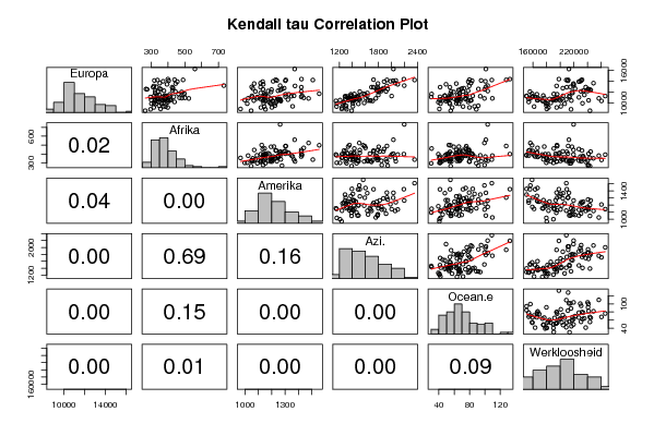
| Title produced by software | Kendall tau Correlation Matrix | ||||||||||||||||||||||||||||||||||||||||||||||||||||||||||||||||||||||||||||||||||||||||||||||||||||||||||||||||||||||||||
| Date of computation | Mon, 15 Dec 2008 14:19:14 -0700 | ||||||||||||||||||||||||||||||||||||||||||||||||||||||||||||||||||||||||||||||||||||||||||||||||||||||||||||||||||||||||||
| Cite this page as follows | Statistical Computations at FreeStatistics.org, Office for Research Development and Education, URL https://freestatistics.org/blog/index.php?v=date/2008/Dec/15/t1229376061flu0q2s28blwxkp.htm/, Retrieved Thu, 16 May 2024 02:41:47 +0000 | ||||||||||||||||||||||||||||||||||||||||||||||||||||||||||||||||||||||||||||||||||||||||||||||||||||||||||||||||||||||||||
| Statistical Computations at FreeStatistics.org, Office for Research Development and Education, URL https://freestatistics.org/blog/index.php?pk=33827, Retrieved Thu, 16 May 2024 02:41:47 +0000 | |||||||||||||||||||||||||||||||||||||||||||||||||||||||||||||||||||||||||||||||||||||||||||||||||||||||||||||||||||||||||||
| QR Codes: | |||||||||||||||||||||||||||||||||||||||||||||||||||||||||||||||||||||||||||||||||||||||||||||||||||||||||||||||||||||||||||
|
| |||||||||||||||||||||||||||||||||||||||||||||||||||||||||||||||||||||||||||||||||||||||||||||||||||||||||||||||||||||||||||
| Original text written by user: | |||||||||||||||||||||||||||||||||||||||||||||||||||||||||||||||||||||||||||||||||||||||||||||||||||||||||||||||||||||||||||
| IsPrivate? | No (this computation is public) | ||||||||||||||||||||||||||||||||||||||||||||||||||||||||||||||||||||||||||||||||||||||||||||||||||||||||||||||||||||||||||
| User-defined keywords | |||||||||||||||||||||||||||||||||||||||||||||||||||||||||||||||||||||||||||||||||||||||||||||||||||||||||||||||||||||||||||
| Estimated Impact | 148 | ||||||||||||||||||||||||||||||||||||||||||||||||||||||||||||||||||||||||||||||||||||||||||||||||||||||||||||||||||||||||||
Tree of Dependent Computations | |||||||||||||||||||||||||||||||||||||||||||||||||||||||||||||||||||||||||||||||||||||||||||||||||||||||||||||||||||||||||||
| Family? (F = Feedback message, R = changed R code, M = changed R Module, P = changed Parameters, D = changed Data) | |||||||||||||||||||||||||||||||||||||||||||||||||||||||||||||||||||||||||||||||||||||||||||||||||||||||||||||||||||||||||||
| - [Kendall tau Correlation Matrix] [] [2008-12-15 21:14:33] [74be16979710d4c4e7c6647856088456] - D [Kendall tau Correlation Matrix] [Kendall tau] [2008-12-15 21:19:14] [5925747fb2a6bb4cfcd8015825ee5e92] [Current] - D [Kendall tau Correlation Matrix] [verband tussen in...] [2008-12-17 19:07:06] [5e74953d94072114d25d7276793b561e] | |||||||||||||||||||||||||||||||||||||||||||||||||||||||||||||||||||||||||||||||||||||||||||||||||||||||||||||||||||||||||||
| Feedback Forum | |||||||||||||||||||||||||||||||||||||||||||||||||||||||||||||||||||||||||||||||||||||||||||||||||||||||||||||||||||||||||||
Post a new message | |||||||||||||||||||||||||||||||||||||||||||||||||||||||||||||||||||||||||||||||||||||||||||||||||||||||||||||||||||||||||||
Dataset | |||||||||||||||||||||||||||||||||||||||||||||||||||||||||||||||||||||||||||||||||||||||||||||||||||||||||||||||||||||||||||
| Dataseries X: | |||||||||||||||||||||||||||||||||||||||||||||||||||||||||||||||||||||||||||||||||||||||||||||||||||||||||||||||||||||||||||
8955.50 356.40 966.20 1235.80 40.60 180144.00 10423.90 394.30 1153.20 1147.10 63.60 173666.00 11617.20 410.90 1328.30 1376.90 66.80 165688.00 9391.10 385.90 1144.50 1157.70 71.50 161570.00 10872.00 523.70 1477.10 1506.00 99.40 156145.00 10230.40 439.10 1234.90 1271.30 78.20 153730.00 9221.00 399.30 1119.10 1240.20 57.20 182698.00 9428.60 372.90 1356.90 1408.30 86.50 200765.00 10934.50 483.20 1217.00 1334.60 66.10 176512.00 10986.00 468.70 1440.50 1601.20 75.00 166618.00 11724.60 498.30 1556.60 1566.40 55.00 158644.00 11180.90 434.40 1303.60 1297.50 66.80 159585.00 11163.20 371.60 1421.50 1487.60 41.40 163095.00 11240.90 408.70 1172.50 1320.90 53.30 159044.00 12107.10 444.50 1422.10 1514.00 71.40 155511.00 10762.30 383.00 1263.00 1290.90 68.20 153745.00 11340.40 388.90 1428.10 1392.50 84.10 150569.00 11266.80 385.10 1347.00 1288.20 94.00 150605.00 9542.70 347.20 1224.20 1304.40 91.40 179612.00 9227.70 315.60 1201.30 1297.80 79.90 194690.00 10571.90 300.90 997.80 1211.00 40.70 189917.00 10774.40 371.20 1248.80 1454.00 60.30 184128.00 10392.80 340.30 1268.60 1405.70 49.10 175335.00 9920.20 301.90 1016.70 1160.80 42.00 179566.00 9884.90 327.40 1194.30 1492.10 54.30 181140.00 10174.50 398.60 1181.80 1263.00 39.30 177876.00 11395.40 379.90 1150.70 1376.30 47.80 175041.00 10760.20 379.70 1247.20 1368.60 74.50 169292.00 10570.10 418.40 1260.60 1427.60 78.80 166070.00 10536.00 367.90 1249.30 1339.80 81.40 166972.00 9902.60 362.50 1223.20 1248.30 66.00 206348.00 8889.00 296.70 1153.00 1309.80 88.80 215706.00 10837.30 343.00 1191.50 1424.00 54.40 202108.00 11624.10 488.30 1303.10 1590.50 75.80 195411.00 10509.00 402.50 1267.10 1423.10 51.60 193111.00 10984.90 500.70 1125.20 1355.30 53.00 195198.00 10649.10 412.80 1322.40 1515.00 62.70 198770.00 10855.70 385.90 1089.20 1385.60 52.30 194163.00 11677.40 461.90 1147.30 1430.00 30.50 190420.00 10760.20 357.40 1196.40 1494.20 49.90 189733.00 10046.20 316.90 1190.20 1580.90 53.80 186029.00 10772.80 339.20 1146.00 1369.80 65.30 191531.00 9987.70 372.30 1139.80 1407.50 62.70 232571.00 8638.70 264.80 1045.60 1388.30 55.40 243477.00 11063.70 325.90 1050.90 1478.50 66.20 227247.00 11855.70 324.10 1117.30 1630.40 67.20 217859.00 10684.50 324.30 1120.00 1413.50 42.40 208679.00 11337.40 318.20 1052.10 1493.80 56.30 213188.00 10478.00 323.40 1065.80 1641.30 44.90 216234.00 11123.90 295.90 1092.50 1465.00 30.00 213586.00 12909.30 425.00 1422.00 1725.10 54.40 209465.00 11339.90 337.80 1367.50 1628.40 47.80 204045.00 10462.20 322.70 1136.30 1679.80 63.60 200237.00 12733.50 430.20 1293.70 1876.00 72.50 203666.00 10519.20 403.80 1154.80 1669.40 82.20 241476.00 10414.90 333.70 1206.70 1712.40 67.90 260307.00 12476.80 358.10 1199.00 1768.80 67.80 243324.00 12384.60 426.70 1265.00 1820.50 65.60 244460.00 12266.70 376.00 1247.10 1776.20 78.10 233575.00 12919.90 312.00 1116.50 1693.70 41.60 237217.00 11497.30 349.30 1153.90 1799.10 64.30 235243.00 12142.00 340.30 1077.40 1917.50 55.90 230354.00 13919.40 455.70 1132.50 1887.20 78.30 227184.00 12656.80 352.30 1058.80 1787.80 69.80 221678.00 12034.10 481.40 1195.10 1803.80 59.30 217142.00 13199.70 731.90 1263.40 2196.40 103.60 219452.00 10881.30 382.20 1023.10 1759.50 109.70 256446.00 11301.20 392.80 1141.00 2002.60 76.30 265845.00 13643.90 351.60 1116.30 2056.80 81.80 248624.00 12517.00 276.50 1135.60 1851.10 99.60 241114.00 13981.10 371.30 1210.50 1984.30 100.60 229245.00 14275.70 439.00 1230.00 1725.30 79.90 231805.00 13435.00 394.40 1136.50 2096.60 49.30 219277.00 13565.70 445.50 1068.70 1792.20 62.70 219313.00 16216.30 560.00 1372.50 2029.90 101.30 212610.00 12970.00 331.80 1049.90 1785.30 101.20 214771.00 14079.90 404.20 1302.20 2026.50 83.30 211142.00 14235.00 489.80 1305.90 1930.80 127.80 211457.00 12213.40 323.90 1173.50 1845.50 103.70 240048.00 12581.00 269.40 1277.40 1943.10 91.50 240636.00 14130.40 319.20 1238.60 2066.80 95.10 230580.00 14210.80 337.60 1508.60 2354.40 109.00 208795.00 14378.50 399.50 1423.40 2190.70 132.60 197922.00 13142.80 316.70 1375.10 1929.60 79.50 194596.00 | |||||||||||||||||||||||||||||||||||||||||||||||||||||||||||||||||||||||||||||||||||||||||||||||||||||||||||||||||||||||||||
Tables (Output of Computation) | |||||||||||||||||||||||||||||||||||||||||||||||||||||||||||||||||||||||||||||||||||||||||||||||||||||||||||||||||||||||||||
| |||||||||||||||||||||||||||||||||||||||||||||||||||||||||||||||||||||||||||||||||||||||||||||||||||||||||||||||||||||||||||
Figures (Output of Computation) | |||||||||||||||||||||||||||||||||||||||||||||||||||||||||||||||||||||||||||||||||||||||||||||||||||||||||||||||||||||||||||
Input Parameters & R Code | |||||||||||||||||||||||||||||||||||||||||||||||||||||||||||||||||||||||||||||||||||||||||||||||||||||||||||||||||||||||||||
| Parameters (Session): | |||||||||||||||||||||||||||||||||||||||||||||||||||||||||||||||||||||||||||||||||||||||||||||||||||||||||||||||||||||||||||
| Parameters (R input): | |||||||||||||||||||||||||||||||||||||||||||||||||||||||||||||||||||||||||||||||||||||||||||||||||||||||||||||||||||||||||||
| R code (references can be found in the software module): | |||||||||||||||||||||||||||||||||||||||||||||||||||||||||||||||||||||||||||||||||||||||||||||||||||||||||||||||||||||||||||
panel.tau <- function(x, y, digits=2, prefix='', cex.cor) | |||||||||||||||||||||||||||||||||||||||||||||||||||||||||||||||||||||||||||||||||||||||||||||||||||||||||||||||||||||||||||