Free Statistics
of Irreproducible Research!
Description of Statistical Computation | |||||||||||||||||||||
|---|---|---|---|---|---|---|---|---|---|---|---|---|---|---|---|---|---|---|---|---|---|
| Author's title | |||||||||||||||||||||
| Author | *Unverified author* | ||||||||||||||||||||
| R Software Module | rwasp_sdplot.wasp | ||||||||||||||||||||
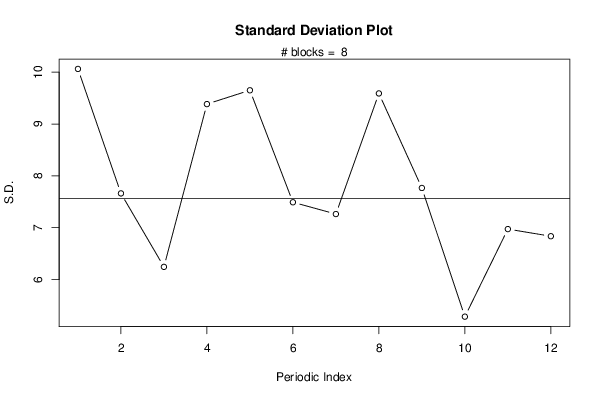
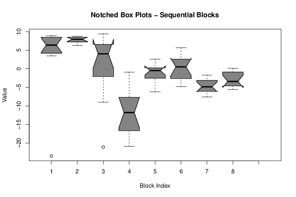
| Title produced by software | Standard Deviation Plot | ||||||||||||||||||||
| Date of computation | Thu, 12 Mar 2015 21:39:53 +0000 | ||||||||||||||||||||
| Cite this page as follows | Statistical Computations at FreeStatistics.org, Office for Research Development and Education, URL https://freestatistics.org/blog/index.php?v=date/2015/Mar/12/t1426196478oo9vufmuiwde0nq.htm/, Retrieved Sat, 18 May 2024 21:28:22 +0000 | ||||||||||||||||||||
| Statistical Computations at FreeStatistics.org, Office for Research Development and Education, URL https://freestatistics.org/blog/index.php?pk=278377, Retrieved Sat, 18 May 2024 21:28:22 +0000 | |||||||||||||||||||||
| QR Codes: | |||||||||||||||||||||
|
| |||||||||||||||||||||
| Original text written by user: | |||||||||||||||||||||
| IsPrivate? | No (this computation is public) | ||||||||||||||||||||
| User-defined keywords | |||||||||||||||||||||
| Estimated Impact | 103 | ||||||||||||||||||||
Tree of Dependent Computations | |||||||||||||||||||||
| Family? (F = Feedback message, R = changed R code, M = changed R Module, P = changed Parameters, D = changed Data) | |||||||||||||||||||||
| - [Standard Deviation Plot] [] [2015-03-12 21:39:53] [70e23d918d09c907c02097a361cd6415] [Current] - RMPD [Variability] [] [2015-05-19 15:47:52] [2f0f353a58a70fd7baf0f5141860d820] - RMPD [Exponential Smoothing] [] [2015-05-19 19:23:10] [2f0f353a58a70fd7baf0f5141860d820] | |||||||||||||||||||||
| Feedback Forum | |||||||||||||||||||||
Post a new message | |||||||||||||||||||||
Dataset | |||||||||||||||||||||
| Dataseries X: | |||||||||||||||||||||
-23,5 5,9 8,4 7,8 4,8 3,5 8,7 6,8 6 3,6 8,7 8,9 8,1 7 7,9 8 7,5 6,3 7,6 8,4 6,8 8,8 8,7 8,7 7,4 2,8 4,8 -21,1 8,5 9,4 1,8 4,8 5,8 3,3 -9 -6 -0,9 -17,3 -9,2 -8,1 -20,9 -14,6 -13,9 -20,8 -16,1 -5 -7,2 -9,7 -1,4 0,2 2,6 -4,8 -6,2 -2 -0,8 -3,1 0,6 0,2 0,3 -0,1 4,3 -3,2 -1,3 1,5 2,5 -2,2 1,7 5,7 2,7 -4,8 -3,1 -0,5 -3,4 -4,7 -5,6 -1,7 -1,8 -5,4 -4,8 -2,8 -4,9 -6,8 -7,6 -6,6 -5,6 -1,4 0,1 -3,7 -5,6 -3,1 -3,8 -5,1 -4,1 -0,3 -0,3 -2,4 | |||||||||||||||||||||
Tables (Output of Computation) | |||||||||||||||||||||
| |||||||||||||||||||||
Figures (Output of Computation) | |||||||||||||||||||||
Input Parameters & R Code | |||||||||||||||||||||
| Parameters (Session): | |||||||||||||||||||||
| par1 = 12 ; | |||||||||||||||||||||
| Parameters (R input): | |||||||||||||||||||||
| par1 = 12 ; | |||||||||||||||||||||
| R code (references can be found in the software module): | |||||||||||||||||||||
par1 <- as.numeric(par1) | |||||||||||||||||||||