Repository of Reproducible Computations

Free Statistics

of Irreproducible Research!

Author's title

Author

*The author of this computation has been verified*

R Software Module

rwasp_autocorrelation.wasp

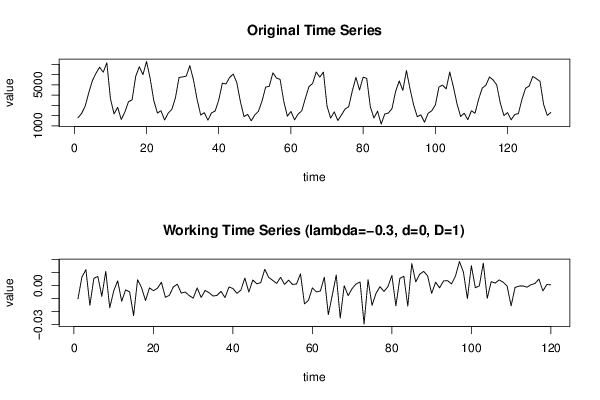
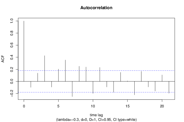
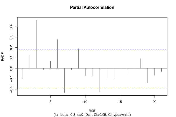
Title produced by software

(Partial) Autocorrelation Function

Date of computation

Wed, 14 Jan 2015 17:11:38 +0000

Cite this page as follows

Statistical Computations at FreeStatistics.org, Office for Research Development and Education, URL https://freestatistics.org/blog/index.php?v=date/2015/Jan/14/t1421255524k8r43bouxequ2hm.htm/, Retrieved Tue, 14 May 2024 01:54:27 +0000

Statistical Computations at FreeStatistics.org, Office for Research Development and Education, URL https://freestatistics.org/blog/index.php?pk=272414, Retrieved Tue, 14 May 2024 01:54:27 +0000

QR Codes:

Paste this QR Code to cite your computation.

Original text written by user:

IsPrivate?

No (this computation is public)

User-defined keywords

Estimated Impact

117

Family? (F = Feedback message, R = changed R code, M = changed R Module, P = changed Parameters, D = changed Data)

-     [Univariate Data Series] [] [2008-12-08 19:22:39] [d2d412c7f4d35ffbf5ee5ee89db327d4]
- RMP   [ARIMA Backward Selection] [] [2011-12-06 19:59:13] [b98453cac15ba1066b407e146608df68]
- RMP     [ARIMA Forecasting] [] [2011-12-06 20:08:12] [b98453cac15ba1066b407e146608df68]
- R         [ARIMA Forecasting] [] [2013-11-22 17:39:30] [0307e7a6407eb638caabc417e3a6b260]
-  MP         [ARIMA Forecasting] [WS 9 arima foreca...] [2014-11-26 14:39:27] [7cbb18b434f1664cf49f28a3db4308dd]
- RMPD            [(Partial) Autocorrelation Function] [] [2015-01-14 17:11:38] [76a64141a2f0df75ca87242b7cc8f1c2] [Current]

Feedback Forum

Post a new message

Dataseries X:

Download CSV

Histogram

Boxplots

Summary of computational transaction
Raw Input	view raw input (R code)
Raw Output	view raw output of R engine
Computing time	1 seconds
R Server	'George Udny Yule' @ yule.wessa.net

\begin{tabular}{lllllllll}
\hline
Summary of computational transaction \tabularnewline
Raw Input & view raw input (R code)  \tabularnewline
Raw Output & view raw output of R engine  \tabularnewline
Computing time & 1 seconds \tabularnewline
R Server & 'George Udny Yule' @ yule.wessa.net \tabularnewline
\hline
\end{tabular}
%Source: https://freestatistics.org/blog/index.php?pk=272414&T=0

[TABLE]
[ROW][C]Summary of computational transaction[/C][/ROW]
[ROW][C]Raw Input[/C][C]view raw input (R code) [/C][/ROW]
[ROW][C]Raw Output[/C][C]view raw output of R engine [/C][/ROW]
[ROW][C]Computing time[/C][C]1 seconds[/C][/ROW]
[ROW][C]R Server[/C][C]'George Udny Yule' @ yule.wessa.net[/C][/ROW]
[/TABLE]
Source: https://freestatistics.org/blog/index.php?pk=272414&T=0

Globally Unique Identifier (entire table): ba.freestatistics.org/blog/index.php?pk=272414&T=0

As an alternative you can also use a QR Code:

The GUIDs for individual cells are displayed in the table below:

Summary of computational transaction
Raw Input	view raw input (R code)
Raw Output	view raw output of R engine
Computing time	1 seconds
R Server	'George Udny Yule' @ yule.wessa.net

Autocorrelation Function
Time lag k	ACF(k)	T-STAT	P-value
1	-0.098066	-1.0743	0.142431
2	0.136879	1.4994	0.068194
3	0.426579	4.6729	4e-06
4	-0.093564	-1.0249	0.153727
5	0.204093	2.2357	0.013609
6	0.354107	3.879	8.6e-05
7	-0.251376	-2.7537	0.003405
8	0.250933	2.7488	0.003453
9	0.237683	2.6037	0.005193
10	-0.19912	-2.1813	0.015557
11	0.231444	2.5353	0.00626
12	-0.092355	-1.0117	0.15686
13	-0.180754	-1.9801	0.024993
14	0.149798	1.641	0.051712
15	0.008744	0.0958	0.461927
16	-0.223117	-2.4441	0.007987
17	0.16646	1.8235	0.03536
18	-0.091117	-0.9981	0.160112
19	-0.159771	-1.7502	0.04132
20	0.107471	1.1773	0.120706
21	-0.196621	-2.1539	0.016625

\begin{tabular}{lllllllll}
\hline
Autocorrelation Function \tabularnewline
Time lag k & ACF(k) & T-STAT & P-value \tabularnewline
1 & -0.098066 & -1.0743 & 0.142431 \tabularnewline
2 & 0.136879 & 1.4994 & 0.068194 \tabularnewline
3 & 0.426579 & 4.6729 & 4e-06 \tabularnewline
4 & -0.093564 & -1.0249 & 0.153727 \tabularnewline
5 & 0.204093 & 2.2357 & 0.013609 \tabularnewline
6 & 0.354107 & 3.879 & 8.6e-05 \tabularnewline
7 & -0.251376 & -2.7537 & 0.003405 \tabularnewline
8 & 0.250933 & 2.7488 & 0.003453 \tabularnewline
9 & 0.237683 & 2.6037 & 0.005193 \tabularnewline
10 & -0.19912 & -2.1813 & 0.015557 \tabularnewline
11 & 0.231444 & 2.5353 & 0.00626 \tabularnewline
12 & -0.092355 & -1.0117 & 0.15686 \tabularnewline
13 & -0.180754 & -1.9801 & 0.024993 \tabularnewline
14 & 0.149798 & 1.641 & 0.051712 \tabularnewline
15 & 0.008744 & 0.0958 & 0.461927 \tabularnewline
16 & -0.223117 & -2.4441 & 0.007987 \tabularnewline
17 & 0.16646 & 1.8235 & 0.03536 \tabularnewline
18 & -0.091117 & -0.9981 & 0.160112 \tabularnewline
19 & -0.159771 & -1.7502 & 0.04132 \tabularnewline
20 & 0.107471 & 1.1773 & 0.120706 \tabularnewline
21 & -0.196621 & -2.1539 & 0.016625 \tabularnewline
\hline
\end{tabular}
%Source: https://freestatistics.org/blog/index.php?pk=272414&T=1

[TABLE]
[ROW][C]Autocorrelation Function[/C][/ROW]
[ROW][C]Time lag k[/C][C]ACF(k)[/C][C]T-STAT[/C][C]P-value[/C][/ROW]
[ROW][C]1[/C][C]-0.098066[/C][C]-1.0743[/C][C]0.142431[/C][/ROW]
[ROW][C]2[/C][C]0.136879[/C][C]1.4994[/C][C]0.068194[/C][/ROW]
[ROW][C]3[/C][C]0.426579[/C][C]4.6729[/C][C]4e-06[/C][/ROW]
[ROW][C]4[/C][C]-0.093564[/C][C]-1.0249[/C][C]0.153727[/C][/ROW]
[ROW][C]5[/C][C]0.204093[/C][C]2.2357[/C][C]0.013609[/C][/ROW]
[ROW][C]6[/C][C]0.354107[/C][C]3.879[/C][C]8.6e-05[/C][/ROW]
[ROW][C]7[/C][C]-0.251376[/C][C]-2.7537[/C][C]0.003405[/C][/ROW]
[ROW][C]8[/C][C]0.250933[/C][C]2.7488[/C][C]0.003453[/C][/ROW]
[ROW][C]9[/C][C]0.237683[/C][C]2.6037[/C][C]0.005193[/C][/ROW]
[ROW][C]10[/C][C]-0.19912[/C][C]-2.1813[/C][C]0.015557[/C][/ROW]
[ROW][C]11[/C][C]0.231444[/C][C]2.5353[/C][C]0.00626[/C][/ROW]
[ROW][C]12[/C][C]-0.092355[/C][C]-1.0117[/C][C]0.15686[/C][/ROW]
[ROW][C]13[/C][C]-0.180754[/C][C]-1.9801[/C][C]0.024993[/C][/ROW]
[ROW][C]14[/C][C]0.149798[/C][C]1.641[/C][C]0.051712[/C][/ROW]
[ROW][C]15[/C][C]0.008744[/C][C]0.0958[/C][C]0.461927[/C][/ROW]
[ROW][C]16[/C][C]-0.223117[/C][C]-2.4441[/C][C]0.007987[/C][/ROW]
[ROW][C]17[/C][C]0.16646[/C][C]1.8235[/C][C]0.03536[/C][/ROW]
[ROW][C]18[/C][C]-0.091117[/C][C]-0.9981[/C][C]0.160112[/C][/ROW]
[ROW][C]19[/C][C]-0.159771[/C][C]-1.7502[/C][C]0.04132[/C][/ROW]
[ROW][C]20[/C][C]0.107471[/C][C]1.1773[/C][C]0.120706[/C][/ROW]
[ROW][C]21[/C][C]-0.196621[/C][C]-2.1539[/C][C]0.016625[/C][/ROW]
[/TABLE]
Source: https://freestatistics.org/blog/index.php?pk=272414&T=1

Globally Unique Identifier (entire table): ba.freestatistics.org/blog/index.php?pk=272414&T=1

As an alternative you can also use a QR Code:

The GUIDs for individual cells are displayed in the table below:

Autocorrelation Function
Time lag k	ACF(k)	T-STAT	P-value
1	-0.098066	-1.0743	0.142431
2	0.136879	1.4994	0.068194
3	0.426579	4.6729	4e-06
4	-0.093564	-1.0249	0.153727
5	0.204093	2.2357	0.013609
6	0.354107	3.879	8.6e-05
7	-0.251376	-2.7537	0.003405
8	0.250933	2.7488	0.003453
9	0.237683	2.6037	0.005193
10	-0.19912	-2.1813	0.015557
11	0.231444	2.5353	0.00626
12	-0.092355	-1.0117	0.15686
13	-0.180754	-1.9801	0.024993
14	0.149798	1.641	0.051712
15	0.008744	0.0958	0.461927
16	-0.223117	-2.4441	0.007987
17	0.16646	1.8235	0.03536
18	-0.091117	-0.9981	0.160112
19	-0.159771	-1.7502	0.04132
20	0.107471	1.1773	0.120706
21	-0.196621	-2.1539	0.016625

Partial Autocorrelation Function
Time lag k	PACF(k)	T-STAT	P-value
1	-0.098066	-1.0743	0.142431
2	0.128497	1.4076	0.080915
3	0.4629	5.0708	1e-06
4	-0.012206	-0.1337	0.446927
5	0.070802	0.7756	0.219755
6	0.277021	3.0346	0.001477
7	-0.232951	-2.5518	0.005986
8	-0.011344	-0.1243	0.450657
9	0.188582	2.0658	0.020499
10	-0.069737	-0.7639	0.223205
11	-0.072968	-0.7993	0.212842
12	-0.227535	-2.4925	0.007024
13	-0.096247	-1.0543	0.146924
14	-0.098806	-1.0824	0.140631
15	0.202466	2.2179	0.014222
16	-0.039816	-0.4362	0.331751
17	0.002154	0.0236	0.490607
18	0.093652	1.0259	0.153499
19	-0.136876	-1.4994	0.068198
20	-0.067187	-0.736	0.231583
21	-0.031735	-0.3476	0.364361

\begin{tabular}{lllllllll}
\hline
Partial Autocorrelation Function \tabularnewline
Time lag k & PACF(k) & T-STAT & P-value \tabularnewline
1 & -0.098066 & -1.0743 & 0.142431 \tabularnewline
2 & 0.128497 & 1.4076 & 0.080915 \tabularnewline
3 & 0.4629 & 5.0708 & 1e-06 \tabularnewline
4 & -0.012206 & -0.1337 & 0.446927 \tabularnewline
5 & 0.070802 & 0.7756 & 0.219755 \tabularnewline
6 & 0.277021 & 3.0346 & 0.001477 \tabularnewline
7 & -0.232951 & -2.5518 & 0.005986 \tabularnewline
8 & -0.011344 & -0.1243 & 0.450657 \tabularnewline
9 & 0.188582 & 2.0658 & 0.020499 \tabularnewline
10 & -0.069737 & -0.7639 & 0.223205 \tabularnewline
11 & -0.072968 & -0.7993 & 0.212842 \tabularnewline
12 & -0.227535 & -2.4925 & 0.007024 \tabularnewline
13 & -0.096247 & -1.0543 & 0.146924 \tabularnewline
14 & -0.098806 & -1.0824 & 0.140631 \tabularnewline
15 & 0.202466 & 2.2179 & 0.014222 \tabularnewline
16 & -0.039816 & -0.4362 & 0.331751 \tabularnewline
17 & 0.002154 & 0.0236 & 0.490607 \tabularnewline
18 & 0.093652 & 1.0259 & 0.153499 \tabularnewline
19 & -0.136876 & -1.4994 & 0.068198 \tabularnewline
20 & -0.067187 & -0.736 & 0.231583 \tabularnewline
21 & -0.031735 & -0.3476 & 0.364361 \tabularnewline
\hline
\end{tabular}
%Source: https://freestatistics.org/blog/index.php?pk=272414&T=2

[TABLE]
[ROW][C]Partial Autocorrelation Function[/C][/ROW]
[ROW][C]Time lag k[/C][C]PACF(k)[/C][C]T-STAT[/C][C]P-value[/C][/ROW]
[ROW][C]1[/C][C]-0.098066[/C][C]-1.0743[/C][C]0.142431[/C][/ROW]
[ROW][C]2[/C][C]0.128497[/C][C]1.4076[/C][C]0.080915[/C][/ROW]
[ROW][C]3[/C][C]0.4629[/C][C]5.0708[/C][C]1e-06[/C][/ROW]
[ROW][C]4[/C][C]-0.012206[/C][C]-0.1337[/C][C]0.446927[/C][/ROW]
[ROW][C]5[/C][C]0.070802[/C][C]0.7756[/C][C]0.219755[/C][/ROW]
[ROW][C]6[/C][C]0.277021[/C][C]3.0346[/C][C]0.001477[/C][/ROW]
[ROW][C]7[/C][C]-0.232951[/C][C]-2.5518[/C][C]0.005986[/C][/ROW]
[ROW][C]8[/C][C]-0.011344[/C][C]-0.1243[/C][C]0.450657[/C][/ROW]
[ROW][C]9[/C][C]0.188582[/C][C]2.0658[/C][C]0.020499[/C][/ROW]
[ROW][C]10[/C][C]-0.069737[/C][C]-0.7639[/C][C]0.223205[/C][/ROW]
[ROW][C]11[/C][C]-0.072968[/C][C]-0.7993[/C][C]0.212842[/C][/ROW]
[ROW][C]12[/C][C]-0.227535[/C][C]-2.4925[/C][C]0.007024[/C][/ROW]
[ROW][C]13[/C][C]-0.096247[/C][C]-1.0543[/C][C]0.146924[/C][/ROW]
[ROW][C]14[/C][C]-0.098806[/C][C]-1.0824[/C][C]0.140631[/C][/ROW]
[ROW][C]15[/C][C]0.202466[/C][C]2.2179[/C][C]0.014222[/C][/ROW]
[ROW][C]16[/C][C]-0.039816[/C][C]-0.4362[/C][C]0.331751[/C][/ROW]
[ROW][C]17[/C][C]0.002154[/C][C]0.0236[/C][C]0.490607[/C][/ROW]
[ROW][C]18[/C][C]0.093652[/C][C]1.0259[/C][C]0.153499[/C][/ROW]
[ROW][C]19[/C][C]-0.136876[/C][C]-1.4994[/C][C]0.068198[/C][/ROW]
[ROW][C]20[/C][C]-0.067187[/C][C]-0.736[/C][C]0.231583[/C][/ROW]
[ROW][C]21[/C][C]-0.031735[/C][C]-0.3476[/C][C]0.364361[/C][/ROW]
[/TABLE]
Source: https://freestatistics.org/blog/index.php?pk=272414&T=2

Globally Unique Identifier (entire table): ba.freestatistics.org/blog/index.php?pk=272414&T=2

As an alternative you can also use a QR Code:

The GUIDs for individual cells are displayed in the table below:

Partial Autocorrelation Function
Time lag k	PACF(k)	T-STAT	P-value
1	-0.098066	-1.0743	0.142431
2	0.128497	1.4076	0.080915
3	0.4629	5.0708	1e-06
4	-0.012206	-0.1337	0.446927
5	0.070802	0.7756	0.219755
6	0.277021	3.0346	0.001477
7	-0.232951	-2.5518	0.005986
8	-0.011344	-0.1243	0.450657
9	0.188582	2.0658	0.020499
10	-0.069737	-0.7639	0.223205
11	-0.072968	-0.7993	0.212842
12	-0.227535	-2.4925	0.007024
13	-0.096247	-1.0543	0.146924
14	-0.098806	-1.0824	0.140631
15	0.202466	2.2179	0.014222
16	-0.039816	-0.4362	0.331751
17	0.002154	0.0236	0.490607
18	0.093652	1.0259	0.153499
19	-0.136876	-1.4994	0.068198
20	-0.067187	-0.736	0.231583
21	-0.031735	-0.3476	0.364361

Figure 1

PNG link

Postscript link

PDF link

Figure 2

PNG link

Postscript link

PDF link

Figure 3

PNG link

Postscript link

PDF link

Parameters (Session):

par1 = 12 ; par2 = Triple ; par3 = additive ;

Parameters (R input):

par1 = Default ; par2 = -0.3 ; par3 = 0 ; par4 = 1 ; par5 = 12 ; par6 = White Noise ; par7 = 0.95 ; par8 = ;

R code (references can be found in the software module):

par8 <- ''
par7 <- '0.95'
par6 <- 'White Noise'
par5 <- '12'
par4 <- '0'
par3 <- '0'
par2 <- '-0.3'
par1 <- 'Default'
if (par1 == 'Default') {
par1 = 10*log10(length(x))
} else {
par1 <- as.numeric(par1)
}
par2 <- as.numeric(par2)
par3 <- as.numeric(par3)
par4 <- as.numeric(par4)
par5 <- as.numeric(par5)
if (par6 == 'White Noise') par6 <- 'white' else par6 <- 'ma'
par7 <- as.numeric(par7)
if (par8 != '') par8 <- as.numeric(par8)
ox <- x
if (par8 == '') {
if (par2 == 0) {
x <- log(x)
} else {
x <- (x ^ par2 - 1) / par2
}
} else {
x <- log(x,base=par8)
}
if (par3 > 0) x <- diff(x,lag=1,difference=par3)
if (par4 > 0) x <- diff(x,lag=par5,difference=par4)
bitmap(file='picts.png')
op <- par(mfrow=c(2,1))
plot(ox,type='l',main='Original Time Series',xlab='time',ylab='value')
if (par8=='') {
mytitle <- paste('Working Time Series (lambda=',par2,', d=',par3,', D=',par4,')',sep='')
mysub <- paste('(lambda=',par2,', d=',par3,', D=',par4,', CI=', par7, ', CI type=',par6,')',sep='')
} else {
mytitle <- paste('Working Time Series (base=',par8,', d=',par3,', D=',par4,')',sep='')
mysub <- paste('(base=',par8,', d=',par3,', D=',par4,', CI=', par7, ', CI type=',par6,')',sep='')
}
plot(x,type='l', main=mytitle,xlab='time',ylab='value')
par(op)
dev.off()
bitmap(file='pic1.png')
racf <- acf(x, par1, main='Autocorrelation', xlab='time lag', ylab='ACF', ci.type=par6, ci=par7, sub=mysub)
dev.off()
bitmap(file='pic2.png')
rpacf <- pacf(x,par1,main='Partial Autocorrelation',xlab='lags',ylab='PACF',sub=mysub)
dev.off()
(myacf <- c(racf$acf))
(mypacf <- c(rpacf$acf))
lengthx <- length(x)
sqrtn <- sqrt(lengthx)
load(file='createtable')
a<-table.start()
a<-table.row.start(a)
a<-table.element(a,'Autocorrelation Function',4,TRUE)
a<-table.row.end(a)
a<-table.row.start(a)
a<-table.element(a,'Time lag k',header=TRUE)
a<-table.element(a,hyperlink('basics.htm','ACF(k)','click here for more information about the Autocorrelation Function'),header=TRUE)
a<-table.element(a,'T-STAT',header=TRUE)
a<-table.element(a,'P-value',header=TRUE)
a<-table.row.end(a)
for (i in 2:(par1+1)) {
a<-table.row.start(a)
a<-table.element(a,i-1,header=TRUE)
a<-table.element(a,round(myacf[i],6))
mytstat <- myacf[i]*sqrtn
a<-table.element(a,round(mytstat,4))
a<-table.element(a,round(1-pt(abs(mytstat),lengthx),6))
a<-table.row.end(a)
}
a<-table.end(a)
table.save(a,file='mytable.tab')
a<-table.start()
a<-table.row.start(a)
a<-table.element(a,'Partial Autocorrelation Function',4,TRUE)
a<-table.row.end(a)
a<-table.row.start(a)
a<-table.element(a,'Time lag k',header=TRUE)
a<-table.element(a,hyperlink('basics.htm','PACF(k)','click here for more information about the Partial Autocorrelation Function'),header=TRUE)
a<-table.element(a,'T-STAT',header=TRUE)
a<-table.element(a,'P-value',header=TRUE)
a<-table.row.end(a)
for (i in 1:par1) {
a<-table.row.start(a)
a<-table.element(a,i,header=TRUE)
a<-table.element(a,round(mypacf[i],6))
mytstat <- mypacf[i]*sqrtn
a<-table.element(a,round(mytstat,4))
a<-table.element(a,round(1-pt(abs(mytstat),lengthx),6))
a<-table.row.end(a)
}
a<-table.end(a)
table.save(a,file='mytable1.tab')

Free Statistics

Description of Statistical Computation

Tree of Dependent Computations

Dataset

Tables (Output of Computation)

Figures (Output of Computation)

Input Parameters & R Code