Free Statistics
of Irreproducible Research!
Description of Statistical Computation | |||||||||||||||||||||
|---|---|---|---|---|---|---|---|---|---|---|---|---|---|---|---|---|---|---|---|---|---|
| Author's title | |||||||||||||||||||||
| Author | *Unverified author* | ||||||||||||||||||||
| R Software Module | rwasp_sdplot.wasp | ||||||||||||||||||||
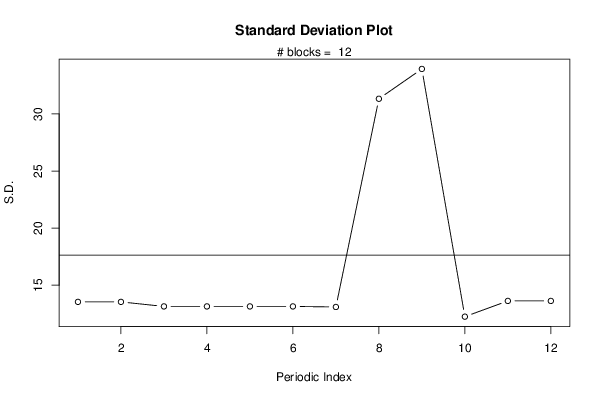
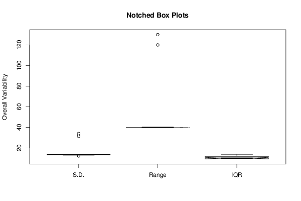
| Title produced by software | Standard Deviation Plot | ||||||||||||||||||||
| Date of computation | Sun, 12 Jan 2014 23:00:23 -0500 | ||||||||||||||||||||
| Cite this page as follows | Statistical Computations at FreeStatistics.org, Office for Research Development and Education, URL https://freestatistics.org/blog/index.php?v=date/2014/Jan/12/t1389585689ecg8ciptfq05euj.htm/, Retrieved Mon, 29 Apr 2024 15:35:08 +0000 | ||||||||||||||||||||
| Statistical Computations at FreeStatistics.org, Office for Research Development and Education, URL https://freestatistics.org/blog/index.php?pk=233101, Retrieved Mon, 29 Apr 2024 15:35:08 +0000 | |||||||||||||||||||||
| QR Codes: | |||||||||||||||||||||
|
| |||||||||||||||||||||
| Original text written by user: | |||||||||||||||||||||
| IsPrivate? | No (this computation is public) | ||||||||||||||||||||
| User-defined keywords | Karel De Grote-Hogeschool Val�rie Weyts | ||||||||||||||||||||
| Estimated Impact | 109 | ||||||||||||||||||||
Tree of Dependent Computations | |||||||||||||||||||||
| Family? (F = Feedback message, R = changed R code, M = changed R Module, P = changed Parameters, D = changed Data) | |||||||||||||||||||||
| - [Bootstrap Plot - Central Tendency] [Bootstrap Plot vo...] [2013-12-29 14:51:21] [ba0d20b2fbb0c8f9ef8b1828cc8a0bda] - RMP [Variability] [variability reeks...] [2013-12-30 12:37:14] [ba0d20b2fbb0c8f9ef8b1828cc8a0bda] - RMPD [Standard Deviation Plot] [Standard Deviaton...] [2014-01-13 04:00:23] [feb2df3f24188fb89c42f3077ec68a56] [Current] | |||||||||||||||||||||
| Feedback Forum | |||||||||||||||||||||
Post a new message | |||||||||||||||||||||
Dataset | |||||||||||||||||||||
| Dataseries X: | |||||||||||||||||||||
80 80 80 80 80 80 80 80 80 80 80 80 80 80 85 85 85 85 85 85 85 85 85 85 85 85 85 85 85 85 85 85 85 85 85 85 90 90 90 90 90 90 90 90 90 90 90 90 90 90 90 90 90 90 90 90 90 90 90 90 90 90 90 90 90 90 90 90 90 90 90 90 90 90 90 90 90 90 90 90 90 90 90 90 90 90 90 90 90 90 90 90 90 90 90 90 90 90 90 90 90 90 100 100 100 100 100 100 100 100 100 100 100 100 100 100 100 110 110 110 110 110 110 110 110 110 110 110 110 110 120 120 120 120 120 120 120 120 120 120 120 120 120 120 120 120 120 120 120 120 120 200 210 | |||||||||||||||||||||
Tables (Output of Computation) | |||||||||||||||||||||
| |||||||||||||||||||||
Figures (Output of Computation) | |||||||||||||||||||||
Input Parameters & R Code | |||||||||||||||||||||
| Parameters (Session): | |||||||||||||||||||||
| par1 = 12 ; | |||||||||||||||||||||
| Parameters (R input): | |||||||||||||||||||||
| par1 = 12 ; | |||||||||||||||||||||
| R code (references can be found in the software module): | |||||||||||||||||||||
par1 <- as.numeric(par1) | |||||||||||||||||||||