Free Statistics
of Irreproducible Research!
Description of Statistical Computation | |||||||||||||||||||||||||||||||||||||||||||||||||||||||||||||
|---|---|---|---|---|---|---|---|---|---|---|---|---|---|---|---|---|---|---|---|---|---|---|---|---|---|---|---|---|---|---|---|---|---|---|---|---|---|---|---|---|---|---|---|---|---|---|---|---|---|---|---|---|---|---|---|---|---|---|---|---|---|
| Author's title | |||||||||||||||||||||||||||||||||||||||||||||||||||||||||||||
| Author | *The author of this computation has been verified* | ||||||||||||||||||||||||||||||||||||||||||||||||||||||||||||
| R Software Module | rwasp_Tests to Compare Two Means.wasp | ||||||||||||||||||||||||||||||||||||||||||||||||||||||||||||
| Title produced by software | T-Tests | ||||||||||||||||||||||||||||||||||||||||||||||||||||||||||||
| Date of computation | Thu, 31 May 2012 12:01:13 -0400 | ||||||||||||||||||||||||||||||||||||||||||||||||||||||||||||
| Cite this page as follows | Statistical Computations at FreeStatistics.org, Office for Research Development and Education, URL https://freestatistics.org/blog/index.php?v=date/2012/May/31/t1338480099p1mrj7n9yb1olb4.htm/, Retrieved Sun, 24 May 2026 12:24:30 +0000 | ||||||||||||||||||||||||||||||||||||||||||||||||||||||||||||
| Statistical Computations at FreeStatistics.org, Office for Research Development and Education, URL https://freestatistics.org/blog/index.php?pk=168106, Retrieved Sun, 24 May 2026 12:24:30 +0000 | |||||||||||||||||||||||||||||||||||||||||||||||||||||||||||||
| QR Codes: | |||||||||||||||||||||||||||||||||||||||||||||||||||||||||||||
|
| |||||||||||||||||||||||||||||||||||||||||||||||||||||||||||||
| Original text written by user: | |||||||||||||||||||||||||||||||||||||||||||||||||||||||||||||
| IsPrivate? | No (this computation is public) | ||||||||||||||||||||||||||||||||||||||||||||||||||||||||||||
| User-defined keywords | |||||||||||||||||||||||||||||||||||||||||||||||||||||||||||||
| Estimated Impact | 350 | ||||||||||||||||||||||||||||||||||||||||||||||||||||||||||||
Tree of Dependent Computations | |||||||||||||||||||||||||||||||||||||||||||||||||||||||||||||
| Family? (F = Feedback message, R = changed R code, M = changed R Module, P = changed Parameters, D = changed Data) | |||||||||||||||||||||||||||||||||||||||||||||||||||||||||||||
| - [Aston University Statistical Software] [Reddy_Moores Wilc...] [2009-11-02 09:28:43] [98fd0e87c3eb04e0cc2efde01dbafab6] - RM [Kolmogorov-Smirnov Test] [Mann-Whitney-Wilc...] [2010-11-02 12:37:15] [98fd0e87c3eb04e0cc2efde01dbafab6] - RM [Wilcoxon-Mann-Whitney Test] [Mann-Whitney-Wilc...] [2010-11-03 14:20:14] [98fd0e87c3eb04e0cc2efde01dbafab6] - RM [Aston University Statistical Software] [Mann-Whitney-Wilc...] [2011-11-01 11:14:29] [72617798859a54657cdee39682e42a20] - RM D [Aston University Statistical Software] [K Test] [2011-11-03 12:42:52] [895f9de29a654334f7aa22b48b6b79ac] - RM D [T-Tests] [T-Test Of Men's r...] [2012-05-31 16:01:13] [40380aa9d3158194c7c2f2fa28deba57] [Current] | |||||||||||||||||||||||||||||||||||||||||||||||||||||||||||||
| Feedback Forum | |||||||||||||||||||||||||||||||||||||||||||||||||||||||||||||
Post a new message | |||||||||||||||||||||||||||||||||||||||||||||||||||||||||||||
Dataset | |||||||||||||||||||||||||||||||||||||||||||||||||||||||||||||
| Dataseries X: | |||||||||||||||||||||||||||||||||||||||||||||||||||||||||||||
182 180 177 175 170 165 167 165 186 180 178 175 171 170 175 174 187 185 197 200 180 178 175 173 173 170 183 180 178 175 173 173 176 175 174 171 178 175 187 188 178 178 183 180 179 175 182 183 169 170 185 185 176 172 183 180 172 169 173 170 165 165 177 170 180 175 189 185 178 175 173 175 182 180 183 183 168 170 182 183 178 175 173 170 184 183 180 180 189 185 185 182 178 175 183 183 179 171 179 179 184 181 184 183 169 165 178 178 178 175 167 165 185 185 177 175 188 185 191 188 175 175 184 183 169 165 172 174 163 161 191 188 169 165 170 170 168 168 178 178 170 165 178 175 174 173 176 175 173 173 183 180 185 188 173 173 175 175 180 180 181 178 177 178 | |||||||||||||||||||||||||||||||||||||||||||||||||||||||||||||
Tables (Output of Computation) | |||||||||||||||||||||||||||||||||||||||||||||||||||||||||||||
| |||||||||||||||||||||||||||||||||||||||||||||||||||||||||||||
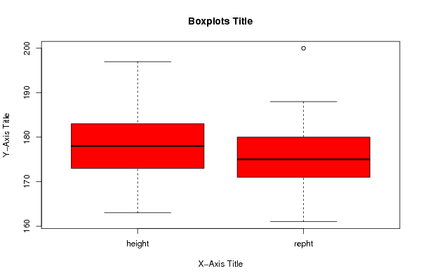
Figures (Output of Computation) | |||||||||||||||||||||||||||||||||||||||||||||||||||||||||||||
Input Parameters & R Code | |||||||||||||||||||||||||||||||||||||||||||||||||||||||||||||
| Parameters (Session): | |||||||||||||||||||||||||||||||||||||||||||||||||||||||||||||
| par1 = two.sided ; par2 = 1 ; par3 = 2 ; | |||||||||||||||||||||||||||||||||||||||||||||||||||||||||||||
| Parameters (R input): | |||||||||||||||||||||||||||||||||||||||||||||||||||||||||||||
| par1 = two.sided ; par2 = 1 ; par3 = 2 ; par4 = T-Test ; par5 = paired ; par6 = 0.0 ; par7 = 0.95 ; par8 = TRUE ; | |||||||||||||||||||||||||||||||||||||||||||||||||||||||||||||
| R code (references can be found in the software module): | |||||||||||||||||||||||||||||||||||||||||||||||||||||||||||||
par8 <- 'TRUE' | |||||||||||||||||||||||||||||||||||||||||||||||||||||||||||||